Community composition of microbial microcosms follows simple assembly rules at evolutionary timescales

Abstract

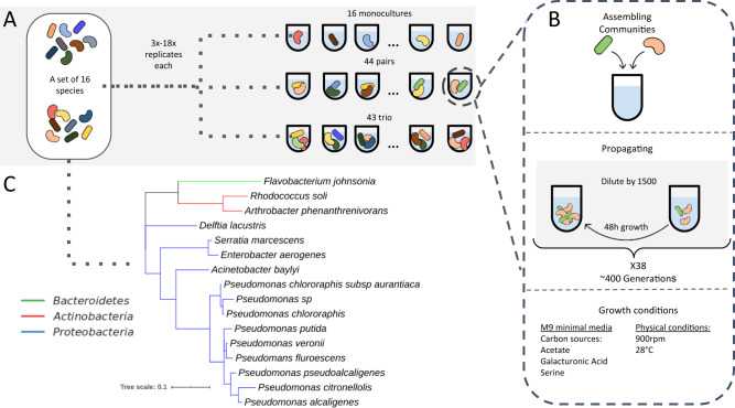
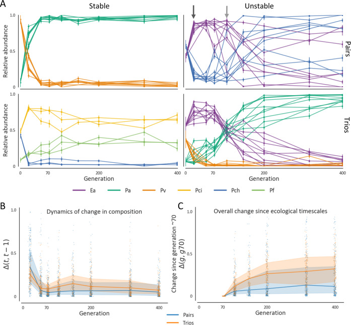
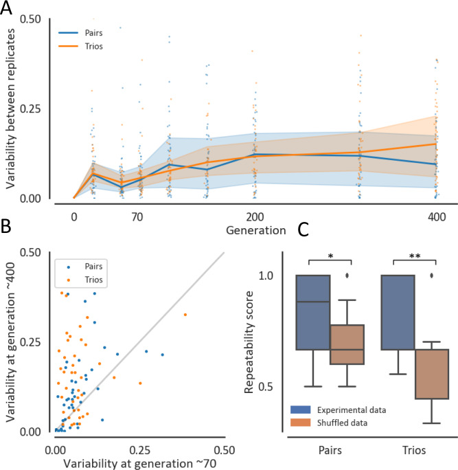
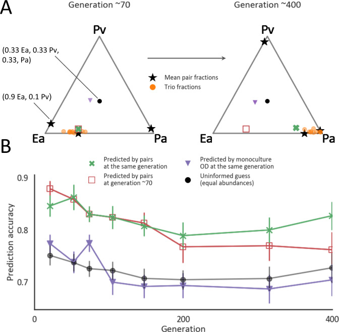
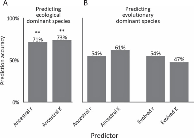
Managing and engineering microbial communities relies on the ability to predict their composition. While progress has been made on predicting compositions on short, ecological timescales, there is still little work aimed at predicting compositions on evolutionary timescales. Therefore, it is still unknown for how long communities typically remain stable after reaching ecological equilibrium, and how repeatable and predictable are changes when they occur. Here, we address this knowledge gap by tracking the composition of 87 two- and three-species bacterial communities, with 3-18 replicates each, for ~400 generations. We find that community composition typically changed during evolution, but that the composition of replicate communities remained similar. Furthermore, these changes were predictable in a bottom-up approach-changes in the composition of trios were consistent with those that occurred in pairs during coevolution. Our results demonstrate that simple assembly rules can hold even on evolutionary timescales, suggesting it may be possible to forecast the evolution of microbial communities.

Fig. 1. A high-throughput evolutionary experiment involving 87 communities composed of subsets of a 16 species set.

A Subsets of the 16 species were used to assemble 44 pairs and 43 trios. All 16 species were evolved in monocultures in parallel to the assembled communities. Each community was grown in 3–18 replicates, a full list of communities and the number of replicates is found in Supplementary Table 2. B Each community was grown in M9 minimal media supplemented with three carbon sources in cycles of 48 h growth-dilution by a factor of 1500. Overall, communities grew for 38 cycles, which correspond to ~400 generations. C Phylogenetic tree based on the full-length 16S sequence of the 16 species used for this study.

Fig. 2. Most communities change significantly during the hundreds of generations following ecological equilibrium.

A Trajectories of the community composition of all replicates of four randomly picked communities representing different levels of stability and repeatability. Colors denote the different species in the community, and different lines are different replicates. Two arrows on the upper-right panel denote the time when most replicates have likely reached an ecological equilibrium (black arrow), and when this equilibrium was disrupted in most replicates (gray arrow). Error bars represent the standard deviation of the posterior beta distribution of the fractions, based on colony counts in each replicate, Error bars were calculated as $\sigma =\frac{\sqrt{p\left(1-p\right)}}{n+1}$, where p is the observed species fraction (colored dot) and n is the total number of colonies counted for a given replicate. For all cases n > 15. B Change in community composition across all communities quantified as the Euclidean distance between the composition of each replicate at two subsequent time points normalized to the maximal distance between two communities composed of n species ($\sqrt{n}$), denoted as $\mathrm{\Delta }\left(t,t-1\right)$. C Change in community composition at evolutionary timescales measured as the Euclidean distance between the composition of each replicate in each time point and its composition at generation ~70 ($\mathrm{\Delta }\left(g,g_{70}\right)$). Generation ~70 is used here as the starting point of the evolutionary timescale since changes in most communities are less rapid after these timescales. For both B and C, blue and orange lines denote the median and shaded areas denote the interquartile range across all pairs and trios, respectively. Source data are provided as a Source Data file.

Fig. 3. Variability between replicate communities increases during ~400 generations, yet remains significantly non-random.

A Variability in community composition between replicate communities is quantified by the mean Euclidean distance of each replicate from the medoid replicate normalized to the maximal distance between two communities composed of n species ($\sqrt{n}$). Blue and orange lines and shaded-areas are the medians and interquartile ranges across all pairs and trios, respectively. Dots denote the variability of specific communities across replicates. B Variability at generation ~400 against ~70, measured as the mean distance from medoid normalized to the maximal distance between two communities composed of n species ($\sqrt{n}$). Each dot represents a pair (blue) or a trio (orange). C Distribution of repeatability scores of the experimental data (38 pairs, 31 trios) and a random null model. The repeatability score is the frequency of replicates in which the same species increased its abundance by the biggest factor between generation ~70 and ~400. Communities that had missing replicates and therefore had less than 3 replicates for either generation ~70 or ~400, were removed from this analysis. The brown boxes represent the distribution of 2000 iterations of a shuffled model, where the values of changes in relative abundances between generation ~70 and ~400 of all species are pooled and are subsequently randomly assigned (for pairs and trios separately) to any species in any community in the dataset. Boxes indicate the quartiles and whiskers are expanded to include values no further than 1.5X interquartile range. *p value = 0.05, **p value <0.005. P values indicate the frequency of iterations were the shuffled data’s mean repeatability score was at least as high as the experimental data’s mean. Source data are provided as a Source Data file.

Fig. 4. Changes in composition that occur in three-species communities are well predicted by those that occur in two-species communities.

A An example predicting the composition of one community at ecological and evolutionary timescales. The trio and the pairwise compositions of the three-species community Ea-Pa-Pv at generation ~70 and ~400. Each triangle is a simplex denoting the fractions of the three species, where each node is a specific species. The black stars on the edges denote the mean fractions in pairwise competition, the orange dots are the compositions of each of the trio replicates. The green cross is the predicted trio composition by pairs at the same generation and the red square, purple triangle, and black dot are predictions made by pairs at generation ~70, species mean carrying capacities at the same generation, and the best-uninformed guess (which means that the species fractions would all be 1/3) respectively. B The accuracy of prediction as $1-\frac{\mathrm{\Delta }\left(\mathrm{prediction},\mathrm{observation}\right)}{\sqrt{\mathrm{n}}}$, where$\mathrm{\Delta }\left(\mathrm{Prediction},\mathrm{Observation}\right)$ is the Euclidean distance between the prediction and the observation and $\sqrt{n}$ is the largest possible distance between two communities with the same n species (here n = 3). Colored markers indicate the mean prediction accuracies of the predictions exemplified in (A), error bars indicate standard errors of 23 trios, and connecting lines help to visualize but do not have a biological meaning. Only trios composed of pairs whose evolutionary trajectories were measured were included in the analysis. Source data are provided as a Source Data file.

Fig. 5. Growth of strains that evolved in monoculture does not predict the dominant species in pairs.

The accuracy of the prediction that the species with the higher growth rate (r)/carrying capacity (K) is more abundant in a pairwise competition at generation ~70 (A) and ~400 (B). Growth rate is measured as the time to a threshold of OD = 0.08 (“Methods”), and thus includes strains’ lag time. An asterisks above bars indicate the probability to get a given level of accuracy by chance (one-sided binomial test, n = 42) ** = <0.001, for bars with no sign the probability is greater than 0.05. P values (from left to right): 0.003, 0.001, 0.32, 0.08, 0.32, 0.67. One species’ growth (H77) was not measured and therefore the two communities that included it were removed from this analysis, and accuracies were evaluated from the data of 42 pairs. Source data are provided as a Source Data file.

References

1. Falkowski PG, Fenchel T, Delong EF. The microbial engines that drive earth’s biogeochemical cycles. Science. 2008;320:1034–1039. - PubMed
1. Gilbert JA, et al. Current understanding of the human microbiome. Nat. Med. 2018;24:392–400. - PMC - PubMed
1. Maukonen J, Saarela M. Microbial communities in industrial environment. Curr. Opin. Microbiol. 2009;12:238–243. - PubMed
1. Huttenhower C, et al. Structure, function and diversity of the healthy human microbiome. Nature. 2012;486:207–214. - PMC - PubMed
1. Sunagawa, S. et al. Structure and function of the global ocean microbiome. Science. 348, 1261359 (2015). - PubMed
Publication types
LinkOut - more resources