. 2021 Jun 10;184(12):3242-3255.e10.
doi: 10.1016/j.cell.2021.04.017. Epub 2021 May 11.

Phase precession in the human hippocampus and entorhinal cortex

Affiliations

Phase precession in the human hippocampus and entorhinal cortex

Salman E Qasim et al. Cell. .

Abstract

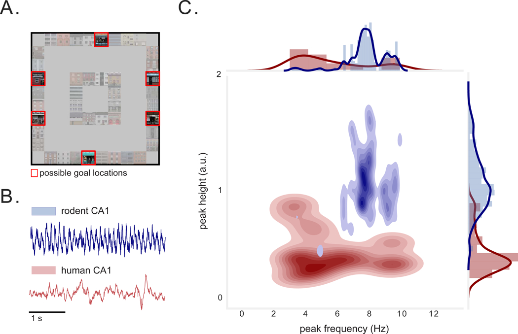
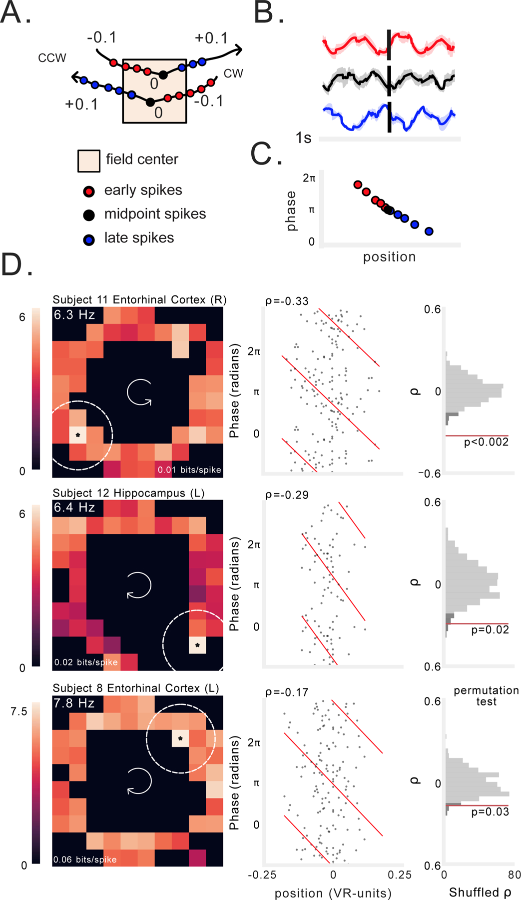
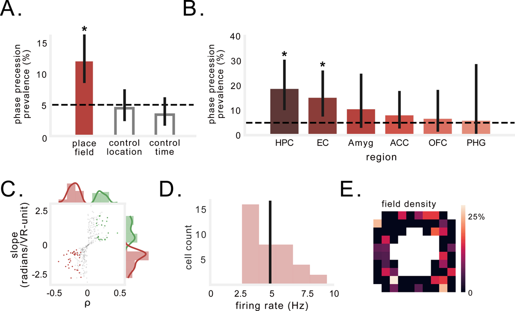
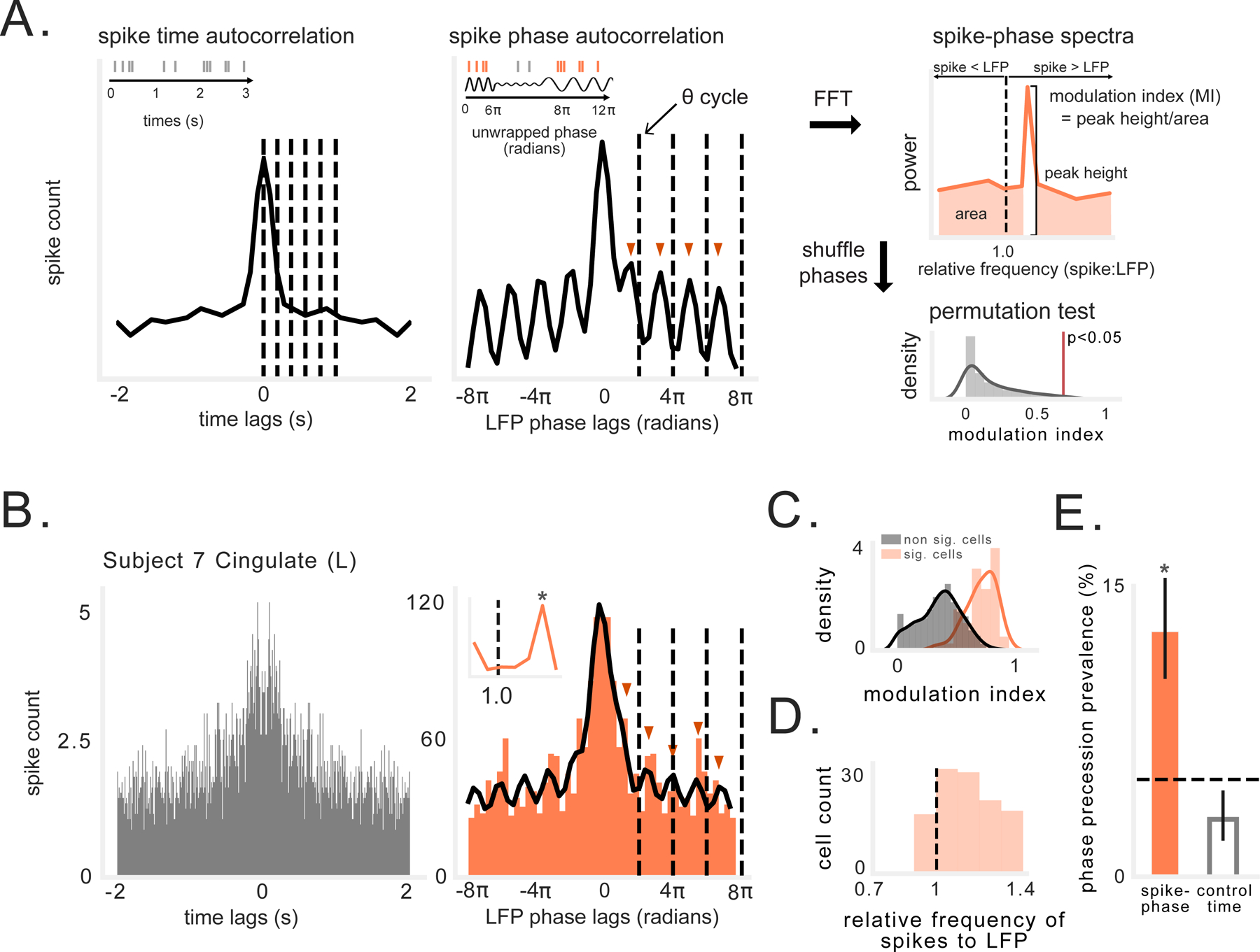
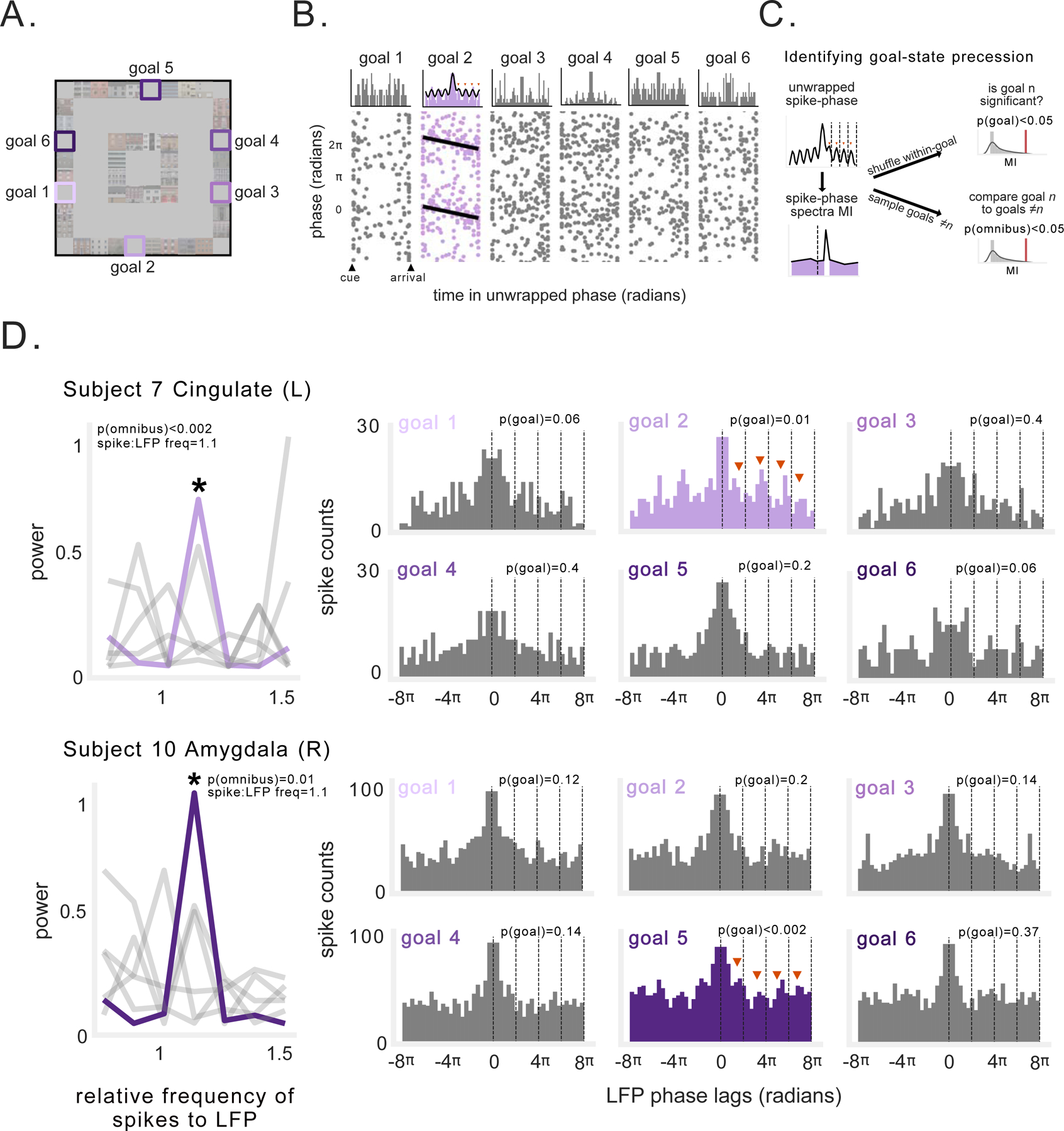
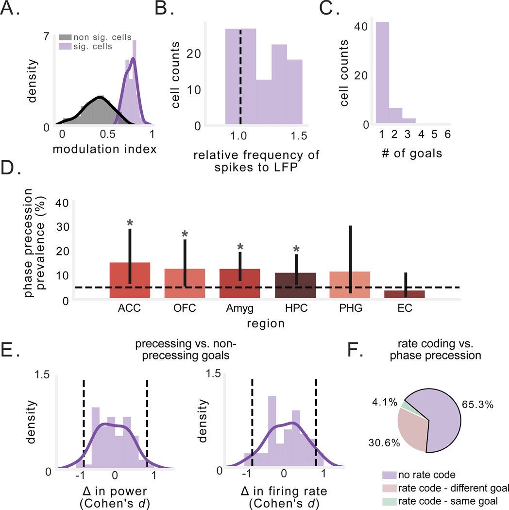
Knowing where we are, where we have been, and where we are going is critical to many behaviors, including navigation and memory. One potential neuronal mechanism underlying this ability is phase precession, in which spatially tuned neurons represent sequences of positions by activating at progressively earlier phases of local network theta oscillations. Based on studies in rodents, researchers have hypothesized that phase precession may be a general neural pattern for representing sequential events for learning and memory. By recording human single-neuron activity during spatial navigation, we show that spatially tuned neurons in the human hippocampus and entorhinal cortex exhibit phase precession. Furthermore, beyond the neural representation of locations, we show evidence for phase precession related to specific goal states. Our findings thus extend theta phase precession to humans and suggest that this phenomenon has a broad functional role for the neural representation of both spatial and non-spatial information.

Keywords: entorhinal cortex; frontal cortex; goal-directed navigation; hippocampus; phase precession; place cells; temporal coding; theta oscillations.


Conflict of interest statement

Declaration of interests The authors declare no competing interests.

Figures

Figure 1:
Figure 1:. Virtual environment and hippocampal local-field potential during task.
A) Overhead view of task environment. Red squares denote locations of possible goal locations. B) Examples of raw LFP data from rodent (publicly available dataset (Mizuseki et al., 2013)) and human hippocampus. C) Joint distribution depicting the peak frequency and peak height of LFP power spectra (PSD) measured from individual rodent (blue) and human (red) hippocampal electrodes. Different electrodes in the rodent hippocampus exhibit highly stereotyped peaks. Human hippocampal recordings exhibit spectral peaks that are significantly smaller in height, and at significantly lower and broader frequencies (p’s < 4×10⁻⁴). See also Figure S1.
Figure 2:
Figure 2:. Examples of spatial phase precession in human hippocampus and entorhinal cortex.
A) Schematic illustrating our method for selecting spikes near peak firing bin (see STAR Methods). For each spatially modulated neuron we analyzed phase precession using spikes that occurred early (red), at the midpoint (black), and late (blue) in clockwise (CW) and counter-clockwise (CCW) trajectories through the center of the firing field. Numbers here denote position relative to the center of the field, in virtual units. B) Spike-triggered average (STA) LFP (reconstructed from phase) for early, midpoint, and late trajectory spikes from one neuron. C) Schematic of spike phase as a function of distance from center spike during a trajectory through the field, showing phase precession as a negative progression of phase-by-position. D) Three examples of spatial phase precession. Each row shows an individual neuron. Left: firing rate heat map. Text label indicates average firing rate in peak firing bin, which is noted with an asterisk, as well as spatial information (bits/spike). Brighter colors denote higher firing rates. Dotted lines indicate maximum radius around field in which spiking was assessed. Arrows in the center of the heatmap indicate the navigation direction. Middle: spike phase as a function of location relative to the field center. Spike phases are duplicated vertically to enable visualization of circular-linear regression (red). Rho indicates circular-linear regression coefficient. Right: statistical assessment of circular-linear regression rho using surrogate distribution of circular-linear regression rho values generated by permutation of spike phases. Red line indicates value of real data. Dark gray shading indicates 95th percentile of surrogate distribution. See also Figure S3.
Figure 3:
Figure 3:. Prevalence and characteristics of spatial phase precession in humans.
A) Percentage of spatially modulated neurons that exhibit phase precession during trajectories through the firing field (filled bar). Grey bars show control analyses of precession relative to alternative locations, or as a function of time, not position, during spiking episodes (see Fig. S4). Black dotted line denotes chance. Solid black line indicates 95% binomial confidence interval. Asterisk indicates significant proportion of spatially modulated cells exhibiting phase precession during trajectories through the firing field (p < 3×10⁻⁶, binomial test). B) Percentage of spatially modulated cells across regions (HPC=hippocampus, EC=entorhinal cortex, Amyg=amygdala, ACC=anterior cingulate cortex, OFC=orbitofrontal cortex, PHG=parahippocampal gyrus). Asterisk indicates significant proportion of cells exhibit phase precession (ps < 0.002, binomial test). C) Distributions of circular–linear correlation-coefficients between spike-phase and location, and regression slopes for neurons with significant negative (red) and positive (green) correlations. Gray dots denote non-significant correlations. D) Distribution of average firing rate of peak firing bins in which phase precession was observed. Black line denotes the mean of the distribution. E) Prevalence of phase precession across the environment. Colors indicate percentage of firing fields in each bin that exhibited precession.
Figure 4:
Figure 4:. Spike-phase spectra reveals precession-like pattern in non-spatially tuned neurons.
A) Schematic illustrating analysis of rhythmic spiking frequency relative to LFP oscillation (see STAR Methods). Left: Envelope of autocorrelation of spike times (gray), with dotted lines at 200 ms intervals. Middle: Envelope of autocorrelation of unwrapped spike phases, using spikes occurring during the oscillation (orange). Dotted lines indicate one cycle of ongoing LFP in 2–10-Hz band. Red arrows indicate peaks in autocorrelation, which occur progressively earlier than cycles of ongoing LFP. Right: Fourier transform (FFT) of autocorrelation function yields power spectral density(PSD) showing cell spiking frequency relative to ongoing LFP frequency. The spike-phase modulation index (MI) is visualized here as the ratio of the spectral peak height to power at all other relative frequencies. This value is compared to a null distribution of MI values generated by shuffling spike phases in each cycle. B) Left: Spike time autocorrelation showing little evidence of theta modulation, which could not be fit with decaying sine wave function (see STAR Methods). Right: Spike phase autocorrelation (orange) showing cell oscillating slightly faster than ongoing LFP (cycles of 2–10 Hz LFP indicated by dotted line). Black line depicts envelope fit using decaying sine wave function (R2 = 0.84). Red arrows indicate peaks in autocorrelation, which occur progressively earlier than cycles of ongoing LFP (and faster than in panel A). Inset shows spike-phase spectra. C) Spike-phase modulation index (MI) of spike-phase spectral peaks for significant vs. non-significant neurons. D) Distribution of relative frequencies for neurons exhibiting significant MI. Values to the right of the black line indicate that the rhythmic spiking frequency slightly exceeded the LFP frequency. E) Percentage of non-spatial cells that exhibit precession-like spiking relative to LFP phase, compared to cell’s exhibiting precession relative to time in a spiking episode. Black dotted line denotes chance level. Solid black line indicates 95% binomial confidence interval. Asterisk indicates significant proportion of cells (p < 7×10⁻¹⁸, binomial test).
Figure 5:
Figure 5:. Goal-state phase precession.
A) Schematic of task environment. Labels indicate goal locations. B) Spike-phases during navigation to different goals for example neuron. Top: unwrapped spike-phase autocorrelograms for each goal. Black line indicates fit of decaying-sine wave function. Spiking frequency transiently exceeded LFP frequency only during navigation to goal 2. Bottom: Spike-phase as a function of duration within each goal epoch. Black line indicates circular-linear regression fit. C) Schematic of method for assessing goal-state phase precession. If a neuron exhibited a significant spike-phase spectral peak at relative frequency exceeding 1 (following multiple comparisons correction), and this effect was significantly stronger than that observed during trajectories to other goals, then this neuron was classified as exhibiting goal-state precession (see STAR Methods). D) Example neurons exhibiting phase precession during navigation to specific goals. Left: Spike-phase spectra depicting frequency of neuronal spiking relative to ongoing LFP. Asterisk denotes spectral peaks that were significant and significantly different from other spike-phase spectra for other goals. Gray lines denote non-significant goals. Right: Spike-phase autocorelograms during navigation to each goal (significant goal epochs depicted in color). Text indicates the p-value for significance tests described in C). See also Figure S5.
Figure 6:
Figure 6:. Prevalence and characteristics of goal-state phase precession in neurons that are not spatially tuned.
A) Spike-phase modulation index (MI) of spike-phase spectral peaks for significant vs. non-significant goals. B) Peak spike-phase PSD frequency for all goals for which a neuron exhibited a significant MI in the spike-phase spectra. Values to the right of the black line indicate that the neuronal frequency slightly exceeded the LFP frequency, indicating precession. C) Number of goals per neuron for which precession was observed. Most neurons exhibited precession during only one goal. D) Percentage of non-spatial cells in each region that exhibited goal-state phase precession. Asterisks indicate significant proportion of cells (p’s < 0.02, binomial test). E) Distribution of Cohen’s d for the difference in 2–10-Hz power (left) and firing rate (right) between trajectories to goals showing precession vs. those that did not. Black dotted lines indicate effect size of ±0.8. F) Analysis of overlap between goal-state phase precession and rate coding for goals.

Comment in

  • Keep time to find your way.
    Schubert T. Schubert T. Nat Rev Neurosci. 2021 Jul;22(7):385. doi: 10.1038/s41583-021-00476-2. Nat Rev Neurosci. 2021. PMID: 34075222 No abstract available.

Similar articles

Cited by

References

    1. Aghajan ZM, Acharya L, Moore JJ, Cushman JD, Vuong C, & Mehta MR (2014). Impaired spatial selectivity and intact phase precession in two-dimensional virtual reality. Nature neuroscience. - PubMed
    1. Aronov D, Nevers R, & Tank DW (2017). Mapping of a non-spatial dimension by the hippocampal–entorhinal circuit. Nature, 543, 719. - PMC - PubMed
    1. Belluscio MA, Mizuseki K, Schmidt R, Kempter R, & Buzsáki G (2012). Cross-frequency phase–phase coupling between theta and gamma oscillations in the hippocampus. Journal of Neuroscience, 32, 423–435. - PMC - PubMed
    1. Benjamini Y & Hochberg Y (1995). Controlling the False Discovery Rate: a practical and powerful approach to multiple testing. Journal of Royal Statistical Society, Series B, 57, 289–300.
    1. Bi G & Poo M (2001). Synaptic modification by correlated activity: Hebb’s postulate revisited. Annu Rev Neurosci, 24, 139–66. - PubMed

Publication types

LinkOut - more resources