Functional interferometric diffusing wave spectroscopy of the human brain

Abstract

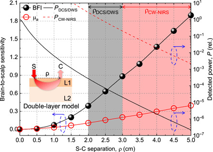
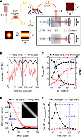
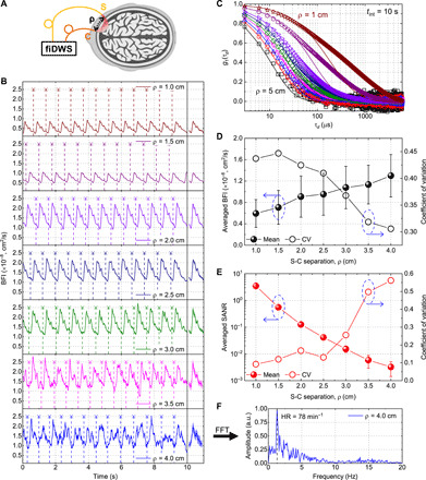
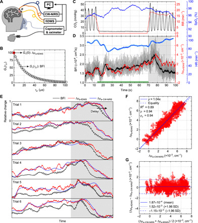
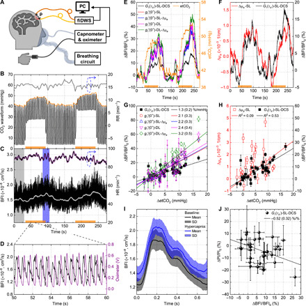
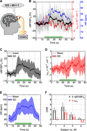
Cerebral blood flow (CBF) is essential for brain function, and CBF-related signals can inform us about brain activity. Yet currently, high-end medical instrumentation is needed to perform a CBF measurement in adult humans. Here, we describe functional interferometric diffusing wave spectroscopy (fiDWS), which introduces and collects near-infrared light via the scalp, using inexpensive detector arrays to rapidly monitor coherent light fluctuations that encode brain blood flow index (BFI), a surrogate for CBF. Compared to other functional optical approaches, fiDWS measures BFI faster and deeper while also providing continuous wave absorption signals. Achieving clear pulsatile BFI waveforms at source-collector separations of 3.5 cm, we confirm that optical BFI, not absorption, shows a graded hypercapnic response consistent with human cerebrovascular physiology, and that BFI has a better contrast-to-noise ratio than absorption during brain activation. By providing high-throughput measurements of optical BFI at low cost, fiDWS will expand access to CBF.

Fig. 1. Brain-to-scalp sensitivity of optical BFI (DCS/DWS) exceeds that of absorption (CW-NIRS).

The brain-to-scalp sensitivities of optical BFI and optical absorption (μ_a) measurements were simulated (section S5) with a double-layer model (inset), with extracerebral and cerebral layers designated as “scalp” and “brain” for short. Optical BFI is intrinsically more brain specific than absorption, achieving a higher brain-to-scalp sensitivity at a given S-C separation. However, the remitted light flux and detected power (right y axis) decrease approximately exponentially with increasing S-C separation, which is needed for high brain-to-scalp sensitivity. Because of the expense of single or few mode photon-counting channels, required for coherence, DCS/DWS uses relatively short S-C separations (black shading). On the other hand, CW-NIRS can collect many modes that sum incoherently and therefore can use larger S-C separations (red shading). We assume that P_{CW − NIRS} is 10⁴ × P_DCS/DWS, based on a hypothetical CW-NIRS system that collects 10⁴ modes for every single DCS/DWS mode. Blue dashed ovals with arrows point to corresponding y axes. Inset: ρ (S-C separation), L1 (extracerebral layer), and L2 (cerebral layer). Note that in practice, effective brain-to-scalp sensitivity can be further improved by considering additional superficial short S-C channels in signal analysis.

Fig. 2. fiDWS for optical BFI in the human brain.

(A) Schematic of fiDWS. The interferometer detection path is shown in both horizontal (H) and vertical (V) views. Transverse intensity distributions of sample and reference light, at positions indicated by red and blue dotted lines, are shown (insets) with correspondingly colored dotted frames. SMF, single-mode fiber; MMF, multimode fiber; L1 to L4, lenses; VOA, variable fiber-optic attenuator; PL, Powell lens; BS, beamsplitter; CL, cylindrical lens. (B) Intensity patterns of reference light used in this work (black) and previous work (45) (red). DN, digital number. (C) Comparisons of estimated N_Speckle (squares and circles) and SANR (triangles) versus width of rectangular window used for pixel binning. Corresponding SANR (for this work), based on optimized pixel binning (fig. S5), is indicated by the spherical symbol. Blue dashed ovals with arrows point to corresponding y axes. (D) Spatial correlation of heterodyne signals across pixels (scatters) and corresponding Gaussian fits (solid curves). Inset shows the correlation matrix of the current system within the gray shaded region in (B). HWHM, half width at half maximum. (E) Comparison of SANR² × N_{Noise speckle}, a metric for fiDWS system performance that is proportional to the autocorrelation SNR. The spherical symbol shows the fiDWS results with optimized data processing (see also section S6 and fig. S5), achieving a ~23.3 times improvement compared to (45). Note that comparisons in (C) to (E) are based on phantom measurements with the same S-C separation.

Fig. 3. fiDWS monitors pulsatile BFI at 3.5-cm S-C separation and autocorrelations at up to 5-cm S-C separation from the adult human forehead.

(A) Schematic of human brain measurements. (B) Pulsatile BFI traces from a single subject with S-C separations from 1 to 4 cm. Temporal sampling and integration time are 0.01 and 0.1 s, respectively. Vertical dashes show estimated boundaries of BFI pulses corresponding to heartbeats. The heartbeat-averaged BFI waveforms [standard deviations (SDs) shaded] follow the BFI traces. (C) Normalized field autocorrelations [g₁(τ_d)] at multiple S-C separations from 1 to 5 cm for the same subject in (B) (open symbols), with an integration time of 10 s. Solid curves show semi-infinite DCS model fits. (D and E) Averaged BFI (D) and SANR (E) versus S-C separation from multiple forehead locations across multiple subjects. Error bars indicate SDs. Corresponding coefficients of variation (CV; right y axes) are shown for averaged BFI (D) and SANR (E). Blue dashed ovals around symbols with arrows point to corresponding y axes. (F) Fast Fourier transform (FFT) spectrum of pulsatile BFI trace at 4-cm S-C separation (B) shows a peak (dashed line) at the HR of 78 min⁻¹. a.u., arbitrary units.

Fig. 4. fiDWS monitors CW light intensity.

(A) Schematic of simultaneous fiDWS and CW-NIRS measurements during voluntary apnea (VA). (B) BFI and absorption can be determined from the noise-corrected field autocorrelation function, G₁(τ_d). (C) CO₂ waveform measured by capnometer and estimated respiration rate (RR) during a single VA trial. Oxygen saturation (SpO₂) was measured by a fingertip pulse oximeter. (D) BFI traces with (gray) and without (black) pulsatility, fitted from G₁(τ_d) with integration times of 0.1 and 2 s, respectively, were derived from a semi-infinite DCS model. Corresponding absorption changes (Δμ_{a − fiDWS}) were estimated from changes in noise-corrected G₁(0) with a 2-s integration time. HR, estimated from pulsatile BFI (blue), agrees with HR measured by the oximeter (light blue). Green bar on x axis indicates the VA period. (E) Rescaled BFI and Δμ_{a − fiDWS} (each normalized to [0, 1]), along with Δμ_{a − CW − NIRS} traces (also normalized), from simultaneous measurements during six VA trials. The resumption of breathing is indicated by the gray shaded area [(D) and (E)], where a clear relative delay of Δμ_a relative to BFI is consistently observed. The falling edge lag between BFI and Δμ_{a − fiDWS}, estimated as the maximum of the unbiased cross-correlation of rescaled waveforms within the gray shaded area, was 3.8 ± 1.6 s. This time lag is consistent with a delayed cerebrovascular “washout” effect (54). Note that the last 15 s of CW-NIRS data was unavailable in trial 3. (F) Scatter plot of Δμ_{a − fiDWS} and Δμ_{a − CW − NIRS} extracted from (E). Solid and dashed blue lines represent proportional fitting (slope of 1.04) and equality, respectively. ρ and ρ_c are Pearson and concordance correlation coefficients, respectively. (G) Bland-Altman plot shows the average (x axis) and difference (y axis) of Δμ_a measured by the two techniques.

Fig. 5. Validation of fiDWS during mild hypercapnia at 3.5-cm S-C separation.

(A) Experimental setup. (B) CO₂ waveform (black) and etCO₂ (orange upper envelope) during two periods of hypercapnia (orange bars along x axis). RR (gray) was estimated from the CO₂ waveform. (C) A single-layer (SL) DCS model with integration times of 0.1 and 10 s, respectively, yielded BFI traces with (black) and without (light gray) pulsatility. HR estimated from pulsatile BFI (black) and oximeter (purple) agrees. (D) Synchronized pulsatile BFI and oximeter traces. (E) Comparison of etCO₂ (right y axis) and BFI, estimated by one of five fitting models: a SL-DCS model, a single-layer $g_1^{\prime }(0^{+})$ (-SL) model without or with (−Δμ_a) absorption compensation, and a double-layer $g_1^{\prime }(0^{+})$ (-DL) model without or with (−Δμ_a) absorption compensation (see Materials and Methods and section S4). (F) Comparison of absorption and BFI determined by single-layer models. (G) Comparison of graded BFI responses to etCO₂ for all five models, across multiple trials and subjects, with proportional fit slopes and 95% confidence intervals in legend. (H) Comparison of graded absorption (SL) and BFI (SL-DCS) responses. Error bars in (G) and (H) indicate SDs within estimation windows (typically, 20 s around falling edge of etCO₂ trace). Solid lines indicate proportional fits (Y = αX) [(G) and (H)]. Note that R² values were estimated from linear fits (Y = αX + β). (I) Heartbeat-averaged BFI at baseline (black) and during hypercapnia (blue), indicated by shaded regions in (C) (SD, shaded SDs). (J) Hypercapnia-induced pulsatility index (PI) changes versus BFI changes from (H). The slope of a proportional fit was −0.52, with a 95% confidence interval of (−0.2 to −0.84). Error bars indicate SDs of ΔBFI/BFI₀ and ΔPI/PI₀.

Fig. 6. fiDWS during prefrontal cortex activation.

(A) Schematic of MA experiments. (B) Single trial changes in BFI with a 0.1-s integration time (light gray), BFI with a 2-s integration time (black), absorption (red), and HR (blue), the latter estimated from a short-time FFT of pulsatile BFI within a 5-s sliding window. The green bar on the x axis indicates the stimulus duration. (C to E) Averaged BFI (C), absorption (D), and HR (E) responses from multiple MA trials for one subject. Shading indicates SDs across trials. (F) The contrast-to-noise ratio (CNR) of BFI exceeds that of absorption for four subjects. Error bars indicate standard errors across trials. All BFIs in this figure were estimated by the SL-DCS model, with no absorption compensation.

References

1. Xing C.-Y., Tarumi T., Liu J., Zhang Y., Turner M., Riley J., Tinajero C. D., Yuan L.-J., Zhang R., Distribution of cardiac output to the brain across the adult lifespan. J. Cereb. Blood Flow Metab. 37, 2848–2856 (2017). - PMC - PubMed
1. Markus H. S., Cerebral perfusion and stroke. J. Neurol. 75, 353–361 (2004). - PMC - PubMed
1. Morotti A., Busto G., Bernardoni A., Marini S., Casetta I., Fainardi E., Association between perihematomal perfusion and intracerebral hemorrhage outcome. Neurocrit. Care 33, 525–532 (2020). - PubMed
1. Bouma G. J., Muizelaar J. P., Cerebral blood flow, cerebral blood volume, and cerebrovascular reactivity after severe head injury. J. Neurotrauma 9 (Suppl. 1), S333–S348 (1992). - PubMed
1. Engquist H., Rostami E., Enblad P., Temporal dynamics of cerebral blood flow during the acute course of severe subarachnoid hemorrhage studied by bedside xenon-enhanced CT. Neurocrit. Care 30, 280–290 (2019). - PMC - PubMed
Publication types