Segmenting surface boundaries using luminance cues

Abstract

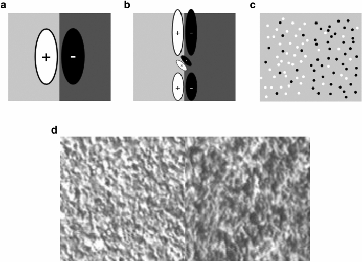
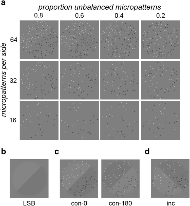
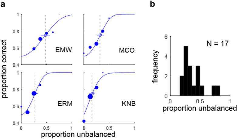
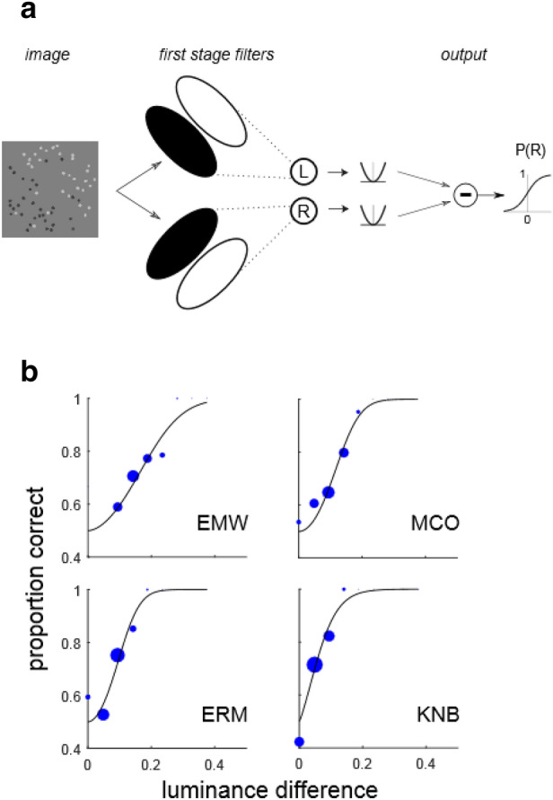
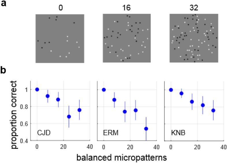
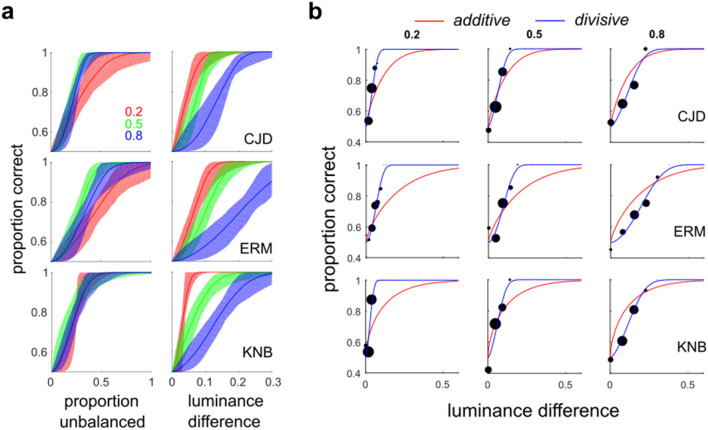
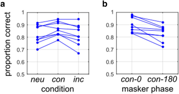
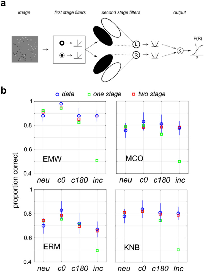
Segmenting scenes into distinct surfaces is a basic visual perception task, and luminance differences between adjacent surfaces often provide an important segmentation cue. However, mean luminance differences between two surfaces may exist without any sharp change in albedo at their boundary, but rather from differences in the proportion of small light and dark areas within each surface, e.g. texture elements, which we refer to as a luminance texture boundary. Here we investigate the performance of human observers segmenting luminance texture boundaries. We demonstrate that a simple model involving a single stage of filtering cannot explain observer performance, unless it incorporates contrast normalization. Performing additional experiments in which observers segment luminance texture boundaries while ignoring super-imposed luminance step boundaries, we demonstrate that the one-stage model, even with contrast normalization, cannot explain performance. We then present a Filter-Rectify-Filter model positing two cascaded stages of filtering, which fits our data well, and explains observers' ability to segment luminance texture boundary stimuli in the presence of interfering luminance step boundaries. We propose that such computations may be useful for boundary segmentation in natural scenes, where shadows often give rise to luminance step edges which do not correspond to surface boundaries.

Figure 1

Boundaries without luminance step edges. (a) A luminance step boundary (LSB) and a simple detection model in which a linear Gabor filter measures the regional luminance difference. (b) Model similar to that in (a) where the LSB is analyzed by multiple Gabor filters at varying spatial scales. (c) Example of luminance texture boundary (LTB). The luminance difference is defined by differing proportions of black and white micropatterns on each side of the boundary, with no sharp luminance change at the boundary. (d) Two juxtaposed textures from the Brodatz database. Although there is clearly a regional difference in luminance, there is no sharp luminance change at the boundary.

Figure 2

Stimulus images. (a) Examples of luminance texture boundary (LTB) stimuli used in this study, shown for varying densities (16, 32, 64 micropatterns on each side of boundary) and proportion unbalanced micropatterns (${\pi }_U$ = 0.2, 0.4, 0.6, 0.8). For all of these example stimulus images, the boundary is right oblique. (b) Luminance step boundary (LSB) stimulus. (c) Stimulus image examples with LTB and LSB having the same orientation (congruent), either phase-aligned (con-0) or opposite-phase (con-180). (d) Example image having superimposed, orthogonal (incongruent) luminance texture (right-oblique) and luminance step (left-oblique) boundaries (inc).

Figure 3

Psychometric functions and threshold distributions. (a) Psychometric functions and fitted functions based on SDT model (blue curves) for four observers (EMW, MCO, ERM, KNB) performing luminance texture boundary (LTB) segmentation (Experiment 1a) as a function of the proportion unbalanced micropatterns (${\pi }_U$), i.e. the proportion of micropatterns not having a same-polarity counterpart on the opposite side of the boundary. The size of each solid dot is proportional to the number of trials obtained at that level, and dashed black lines denote 75% thresholds for the fitted curves. Circles and lines indicate threshold estimates and 95% confidence intervals obtained from 200 bootstrapped re-samplings of the data. (b) Histogram of segmentation thresholds (${\pi }_U$) measured from all observers (N = 17) in Experiment 1a.

Figure 4

Single-stage filter model. (a) Image-computable model with a single stage of filtering (IC-1). Luminance differences are computed across the left-oblique and right-oblique diagonals, passed through a rectifying, exponentiating nonlinearity and subtracted to determine the probability P(R) of observer classifying the boundary as right-oblique. In the case where there is only a luminance difference across one diagonal, this model is equivalent to the IC-SDT model (Eq. (4)). (b) Fits of the model in (a) to LTB segmentation data from Experiment 1a for the same observers as in Fig. 3a.

Figure 5

Holding luminance difference constant. (a) Examples of LTB stimuli used in Experiment 2, having an equal number (8) of unbalanced micropatterns on each side of the boundary, with varying numbers (0, 16, 32) of balanced micro-patterns. In this series, the luminance difference across the boundary is constant for all stimuli. (b) Proportion correct responses for three observers for differing numbers of balanced micropatterns. Lines indicate 95% binomial proportion confidence intervals for each level (N = 50 trials at each level). We see that performance degrades significantly with increasing numbers of balanced micropatterns, despite constant luminance difference. This suggests that a simple luminance difference computation may be inadequate to explain segmentation of LTB stimuli.

Figure 6

Using micro-pattern amplitude to vary global luminance difference. (a) Bootstrapped SDT psychometric function fits (200 bootstrapped re-samplings) with 90% confidence intervals of observer performance as a function of proportion unbalanced micropatterns (left panels) and absolute luminance difference (right panels). This shows that identical luminance differences give rise to significantly different levels of observer performance for the three Michaelson contrasts (right panels), i.e. global luminance difference is a very poor predictor of performance. Instead, observer performance is much better predicted by the proportion of unbalanced micro-patterns, (almost) irrespective of micro-pattern amplitude (left panels). (b) Data from Experiment 3 (black dots) and fits of the additive (red) and divisive (blue) image-computable signal detection theory models (IC-SDT) to the data. Each observer was tested at three different maximum micro-pattern amplitudes, which correspond to different Michaelson contrasts (0.2, 0.4, 0.8) of the stimuli. We see that a model incorporating a global luminance difference computation followed by contrast normalization (blue) provides an excellent fit to this data.

Figure 7

Effects of masking LSBs on LTB segmentation. (a) Performance for N = 9 observers in Experiment 4a, segmenting LTB stimuli using a proportion of unbalanced micro-patterns (${\pi }_U$), set at 75% JND for each observer, as measured in Experiment 1a. We see similar performance for most observers in the absence of a masker (neutral case, neu) as well as with a masker having congruent (con) and incongruent (inc) orientation. Here the congruent case pools across in-phase and opposite-phase conditions. (b) Performance for same observers for congruent stimuli which are in-phase (con-0) and opposite-phase (con-180).

Figure 8

Two-stage model fits Experiment 4 results. (a) Model with two cascaded stages of filtering (IC-2). The first stage of this model detects texture elements (here, micro-patterns) on a fine spatial scale. The second stage looks for differences in the outputs of these first-stage filters on the coarse spatial scale of the texture boundary, at either of two possible orientations. Such a model can detect differences in the proportions of black and white micro-patterns on opposite sides of the boundary, while being fairly robust to interference from luminance steps. (b) Fits of single-stage model IC-1 (green squares) and two-stage model IC-2 (red squares) to data from Experiment 4a (blue circles, lines denote 95% confidence intervals), for four ways of combining LTB and LSB stimuli: neutral (neu); congruent, in-phase (c0); congruent, opposite phase (c180); and incongruent (inc).

References

1. Mély DA, Kim J, McGill M, Guo Y, Serre T. A systematic comparison between visual cues for boundary detection. Vision. Res. 2016;120:93–107. doi: 10.1016/j.visres.2015.11.007. - DOI - PubMed
1. DiMattina C, Fox SA, Lewicki MS. Detecting natural occlusion boundaries using local cues. J. Vis. 2012;12(13):15–15. doi: 10.1167/12.13.15. - DOI - PMC - PubMed
1. Martin DR, Fowlkes CC, Malik J. Learning to detect natural image boundaries using local brightness, color, and texture cues. IEEE Trans. Pattern Anal. Mach. Intell. 2004;26(5):530–549. doi: 10.1109/TPAMI.2004.1273918. - DOI - PubMed
1. Marr D. Vision: A Computational Investigation into the Human Representation and Processing of Visual Information. Henry Holt and Co., Inc.; 1982.
1. Hubel DH, Wiesel TN. Receptive fields, binocular interaction and functional architecture in the cat's visual cortex. J. Physiol. 1962;160(1):106. doi: 10.1113/jphysiol.1962.sp006837. - DOI - PMC - PubMed
Publication types
LinkOut - more resources