Reconstruction of ancient microbial genomes from the human gut

Abstract

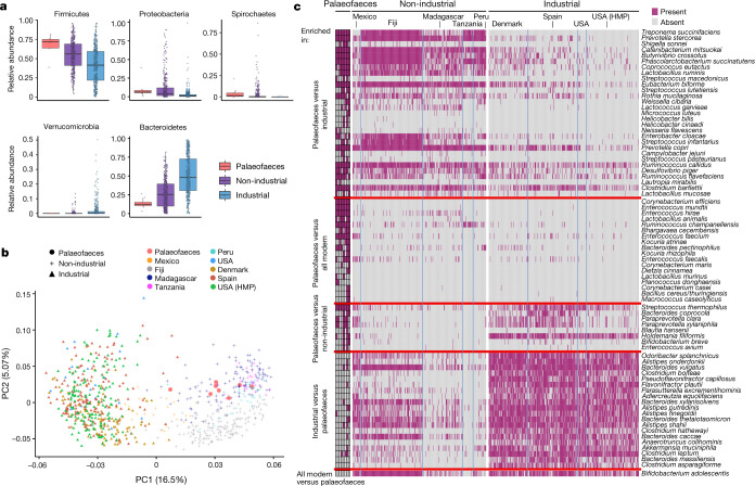
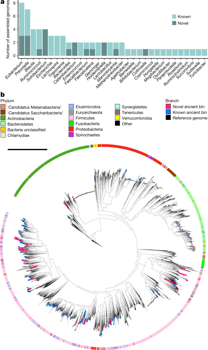
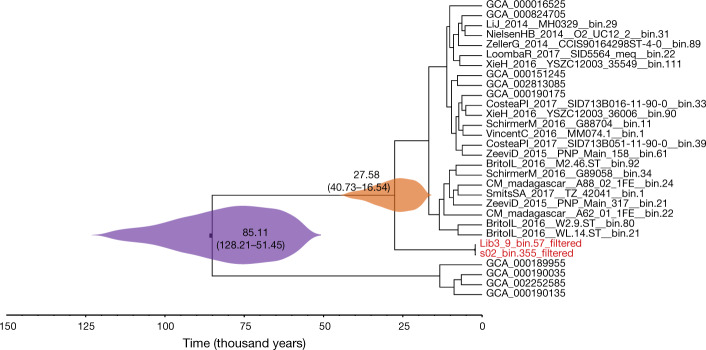
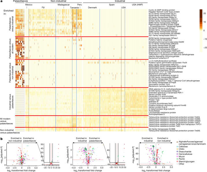
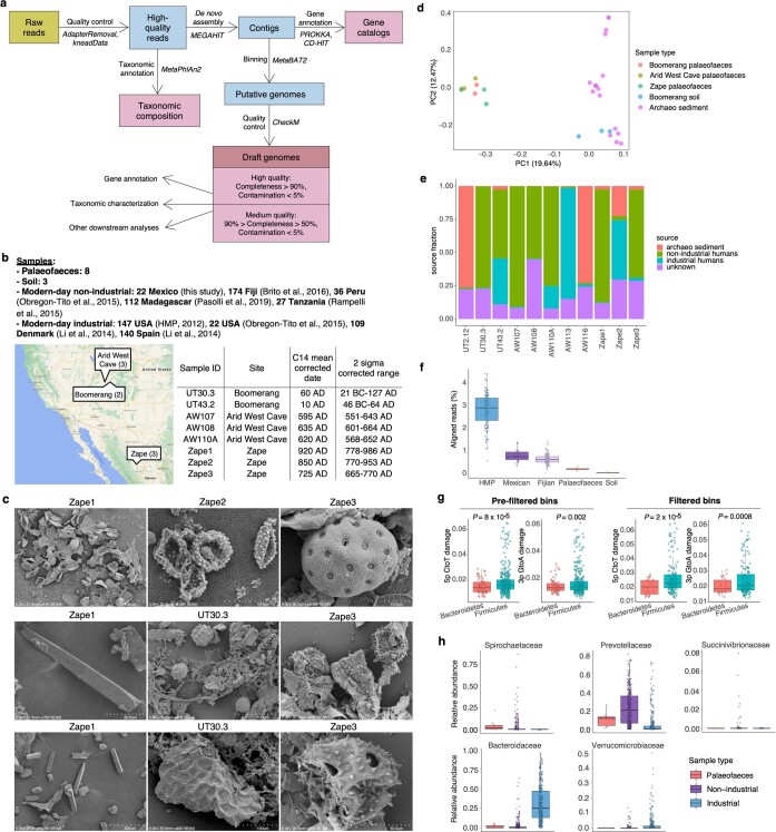
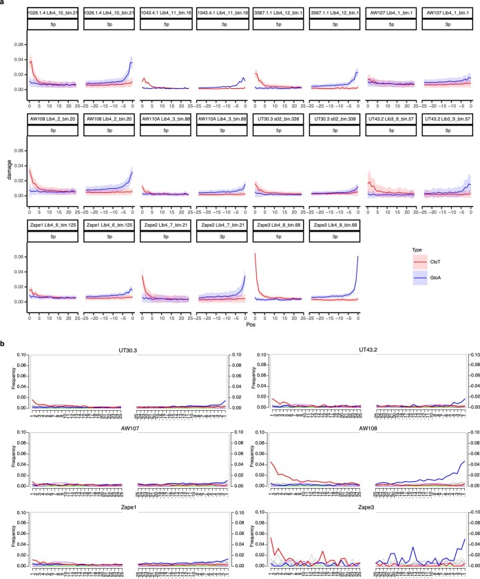
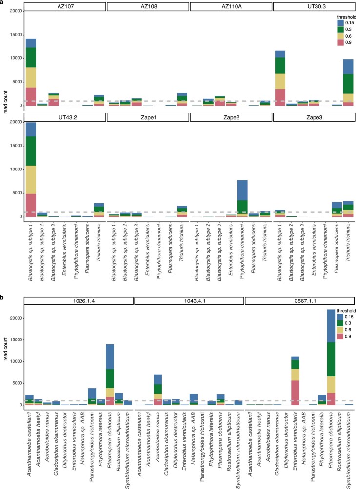
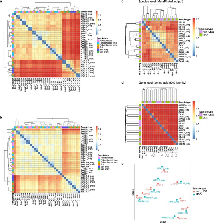
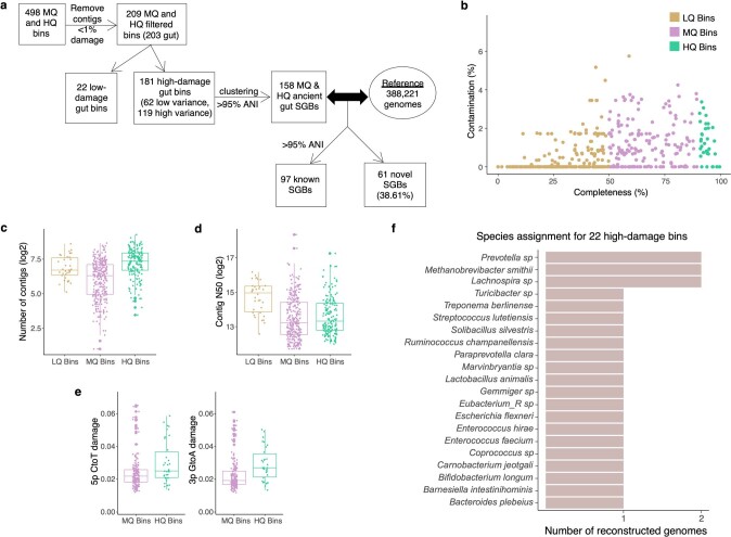
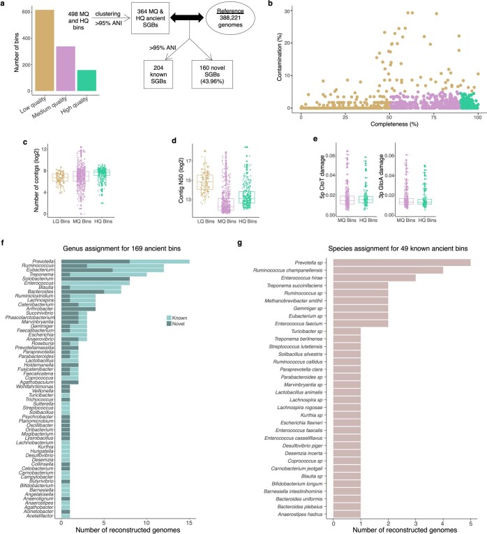
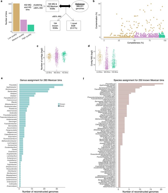
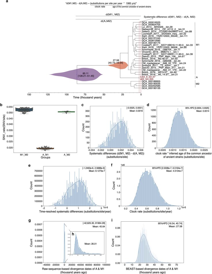
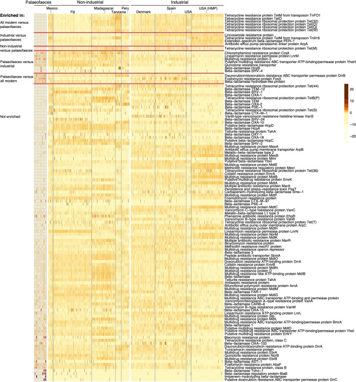
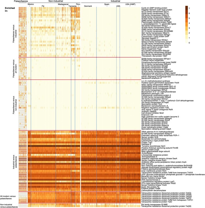
Loss of gut microbial diversity^1-6 in industrial populations is associated with chronic diseases⁷, underscoring the importance of studying our ancestral gut microbiome. However, relatively little is known about the composition of pre-industrial gut microbiomes. Here we performed a large-scale de novo assembly of microbial genomes from palaeofaeces. From eight authenticated human palaeofaeces samples (1,000-2,000 years old) with well-preserved DNA from southwestern USA and Mexico, we reconstructed 498 medium- and high-quality microbial genomes. Among the 181 genomes with the strongest evidence of being ancient and of human gut origin, 39% represent previously undescribed species-level genome bins. Tip dating suggests an approximate diversification timeline for the key human symbiont Methanobrevibacter smithii. In comparison to 789 present-day human gut microbiome samples from eight countries, the palaeofaeces samples are more similar to non-industrialized than industrialized human gut microbiomes. Functional profiling of the palaeofaeces samples reveals a markedly lower abundance of antibiotic-resistance and mucin-degrading genes, as well as enrichment of mobile genetic elements relative to industrial gut microbiomes. This study facilitates the discovery and characterization of previously undescribed gut microorganisms from ancient microbiomes and the investigation of the evolutionary history of the human gut microbiota through genome reconstruction from palaeofaeces.

Fig. 1. Phylum, family and species compositions of the palaeofaeces samples are similar to the gut microbiomes of present-day non-industrial individuals.

a, Differentially abundant phyla (one-tailed Wilcoxon rank-sum test with FDR correction) as identified by MetaPhlAn2 (palaeofaeces, n = 8; non-industrial, n = 370; industrial, n = 418). Data are presented as box plots (middle line, median; lower hinge, first quartile; upper hinge, third quartile; lower whisker, the smallest value at most 1.5× the interquartile range from the hinge; upper whisker, the largest value no further than 1.5× the interquartile range from the hinge; data beyond the whiskers are outlying points). b, Principal component analysis of the species composition as identified by MetaPhlAn2. HMP, Human Microbiome Project. c, Presence–absence heat map (fuchsia, present; grey, absent) for differentially enriched species (two-tailed Fisher’s test, FDR correction). Species without fully specified species names are not shown (a complete list is included in Supplementary Table 3).

Fig. 2. De novo genome reconstruction from palaeofaeces recovers 181 authenticated ancient gut microbial genomes, 39% of which are novel SGBs.

a, GTDB-Tk genus estimation for both novel and known species. b, Maximum likelihood tree of 178 highly damaged filtered ancient gut bacteria and 4,930 representative human gut microbiome genomes. The tree was constructed using multiple sequence alignment of 120 bacterial marker genes identified by GTDB-Tk. Novel and known ancient bin branches are highlighted in pink and blue, respectively. Tree scale, 1 nucleotide substitution per site.

Fig. 3. Evolutionary context of a key human gut symbiont.

A time-measured phylogenetic tree of M. smithii reconstructed on the basis of the core genome using a Bayesian approach under a strict clock model. Purple and orange violin plots illustrate the 95% HPD values (in parentheses) of estimated mean ages for the diversification of M. smithii and the split of the lineage leading to ancient M. smithii (highlighted in red), respectively.

Fig. 4. Palaeofaeces exhibit a distinct functional genomic repertoire compared to present-day industrial stool samples.

a, Heat map of the top-15 genes enriched in the palaeofaeces, industrial and non-industrial samples (complete results in Supplementary Table 8). Functions were annotated using PROKKA (one-tailed Wilcoxon rank-sum tests with Bonferroni correction). The reads per kilobase per million reads (RPKM) values shown are on a log scale and scaled by row. An unscaled heat map is shown in Extended Data Fig. 12. b, Volcano plots showing enriched CAZymes signatures (two-tailed Wilcoxon rank-sum test with FDR correction) comparing palaeofaeces and non-industrial samples (left), palaeofaeces and industrial samples (middle), and non-industrial and industrial samples (right). Each data point represents a CAZy family. CAZymes are colour-coded according to manually annotated broad substrate categories. The horizontal dashed red line indicates adjusted P = 0.05. The vertical dashed red line indicates log₂-transformed fold change = 0. For the left and middle plots, both the entire dataset and a magnified version are shown. For the right plot, the x-axis limits were set to −5 and 5 (as a result, eight statistically non-significant CAZymes were removed).

Extended Data Fig. 1. Overview of samples, study design and quality measures to validate the authenticity of the palaeofaeces.

a, Schematic of gene-catalogue and genome-reconstruction pipelines. b, Samples used in this study, archaeological sites and ¹⁴C dating. Data were obtained from this study (Mexico) and previous studies: Fiji, Peru, Madagascar, Tanzania, USA^,, Denmark and Spain. Map data are from Google Maps (2021 Google, INEGI). c, Scanning electron microscopy images of dietary remains in the palaeofaeces. Zape1, maize pollen grains (more than 191,000 grains per gram) (top) and agave phytoliths (middle and bottom). Zape2, U. maydis spores (hundreds of millions per gram). Zape3, Chenopod or amaranth foliage and/or buds (smaller pollen) and squash (larger pollen with spines). UT30.3, druse phytoliths, annular xylem vessel secondary wall thickenings and epidermis of Cactaceae. A complete description is provided in Supplementary Information section 2. Reproducibility and independently repeated experiments are described in the Methods. d, Principal component analysis of the species composition of palaeofaeces, soil samples and publicly available archaeological sediment samples^,. Species were identified by MetaPhlAn2. e, Prediction of source of microbial communities by SourceTracker2 using the species abundance matrix from MetaPhlAn2 as input. Archaeological sediment samples included three soil samples collected in this study, seven Holocene human-associated sediments from CoproID and 40 Pleistocene sediment samples. f, The percentage of reads aligned to the MetaPhlAn2 database per sample (HMP, n = 146; Mexican, n = 22; Fijian, n = 174; palaeofaeces, n = 8; soil, n = 3) (Supplementary Information section 4). g, aDNA damage levels of Firmicutes and Bacteroidetes genomes for medium-quality and high-quality pre-filtered and filtered bins (two-tailed Wilcoxon rank-sum test; pre-filtered bins Bacteroidetes, n = 69 MAGs; pre-filtered bins Firmicutes, n = 359 MAGs; filtered bins Bacteroidetes, n = 24 MAGs; filtered bins Firmicutes, n = 161 MAGs) (Supplementary Information section 5). 5p, 5′ end; 3p, 3′ end. h, Abundances of VANISH and BloSSUM families as identified by MetaPhlAn2 (palaeofaeces n = 8; non-industrial n = 370; industrial n = 418). In f–h, data are presented as box plots (middle line, median; lower hinge, first quartile; upper hinge, third quartile; upper whisker extends from the hinge to the largest value no further than 1.5× the interquartile range from the hinge; lower whisker extends from the hinge to the smallest value at most 1.5× the interquartile range from the hinge; data beyond the end of the whiskers are individually plotted outlying points).

Extended Data Fig. 2. Microbial DNA and mtDNA damage patterns.

a, Microbial damage patterns of the palaeofaeces and the Boomerang soil samples as identified by DamageProfiler. A medium-quality or high-quality reconstructed genome was used as reference for its respective sample. All MAGs used as reference genomes for the palaeofaeces are of known gut microbial species. The red line indicates the average frequency of C-to-T substitutions across all contigs per bin and the blue line indicates the average frequency of G-to-A substitutions across all contigs per bin. The shaded areas show the s.d. (1026.1.4 Lib4_10_bin.21, n = 488 contigs; 1043.4.1 Lib4_11_bin.16, n = 133 contigs; 3567.1.1 Lib4_12_bin.1, n = 278 contigs; AW107 Lib4_1_bin.1, n = 208 contigs; AW108 Lib4_2_bin.20, n = 337 contigs; AW110A Lib4_3_bin.88, n = 210 contigs; UT30.3 s02_bin.338, n = 74 contigs; UT43.2 Lib3_9_bin.57, n = 174 contigs; Zape1 Lib4_6_bin.125, n = 212 contigs; Zape2 Lib4_7_bin.21, n = 241 contigs; Zape3 Lib4_8_bin.68, n = 324 contigs). Contigs with fewer than 1,000 reads aligned were removed from the analysis. b, mtDNA damage patterns of the palaeofaeces as identified by mapDamage2.0. Human mtDNA (rCRS) was used as reference. The red line indicates the average frequency of C-to-T substitutions and the blue line indicates the average frequency of G-to-A substitutions. Samples AW110A and Zape2 did not have enough mtDNA reads for mtDNA damage assessment.

Extended Data Fig. 3. Parasites in the palaeofaeces and the soil samples classified using Kraken 2.

The bars represent the reads assigned with a Kraken confidence threshold between 0.15 and 0.9. The value specifies the fraction of k-mers needed for the specific classification level. The grey dotted line indicates the 1,000 reads cut-off. The displayed parasites were detected above the cut-off in at least one sample. a, Parasites in the palaeofaeces. In six out of eight palaeofaeces samples, Blastocystis is above the cut-off. Subtype 1 is the dominant subtype in samples AW107, UT30.3, UT43.2 and Zape3, whereas subtype 3 is the dominant subtype in AW108 and AW110A. Other parasites do not meet the cut-off requirements described in the Methods. b, Parasites in the soil samples include Acanthamoeba (a parasite frequently found in soil) in sample 1026.1.4 and Enterobius vermicularis (human pinworm) in sample 3567.1.1.

Extended Data Fig. 4. BioAnalyzer results showing the length distribution of DNA fragments per library.

The libraries contain 120-bp adapters.

Extended Data Fig. 5. Species and gene content of long versus short DNA fragments and UDG-treated versus non-UDG-treated samples.

a, b, Pairwise comparison between whole samples, only subsets containing short reads and only subsets with long reads. a, Heat map of species-level pairwise Jaccard distances for whole samples, short-read subsets (reads ≤ 145 bp) and long-read subsets (reads > 145 bp). Species were identified by MetaPhlAn2. The groups cluster together by sample. b, Heat map of gene-level pairwise Jaccard distances for whole samples, short-read subsets and long-read subsets. Genes were identified by PROKKA and a count matrix was built from PROKKA output files. Groups from the same sample cluster together. c–e, Species and gene content comparison between UDG-treated libraries and non-UDG-treated libraries (Supplementary Information section 12 and Supplementary Table 10). c, Heat map of species-level pairwise Jaccard distances between each pair of all UDG-treated and non-UDG-treated samples. Species were identified by MetaPhlAn2. Each UDG-treated library clusters with non-UDG-treated library from the same sample. d, Heat map of gene-level pairwise Jaccard distances between each pair of all UDG-treated and non-UDG-treated samples. Genes were identified by PROKKA and non-redundant gene catalogues were generated by collapsing genes within 10% amino acid identity distance. Each UDG-treated library clusters with non-UDG-treated library from the same sample. e, t-Distributed stochastic neighbour embedding (t-SNE) analysis at the species level shows clustering of each UDG-treated library with the non-UDG-treated library from the same sample.

Extended Data Fig. 6. De novo genome reconstruction from palaeofaeces recovers 181 authenticated ancient gut microbial genomes, 39% of which are novel SGBs.

Related to Fig. 2. a–d, CheckM quality estimation for de novo reconstructed microbial genomes for the 209 filtered bins (low-quality bins, n = 285; medium-quality bins, n = 175; high-quality bins, n = 34). Genomes were classified as low quality (LQ; completeness ≤ 50% or contamination > 5%), medium quality (MQ; 90% ≥ completeness > 50%, contamination < 5%) or high quality (HQ; completeness > 90% and contamination < 5%). a, Filtering steps, number of bins that belong to each of the quality categories and classification of novel SGBs. b, Contamination and completeness distribution for the filtered bins. c, Distribution of the number of contigs for each of the quality categories. d, Distribution of contig N50 values for each of the quality categories. e, Damage levels, specifically C-to-T substitutions at the 5′ end and G-to-A substitutions at the 3′ end of the reads, for each ancient bin as estimated by DamageProfiler (medium-quality bins, n = 175; high-quality bins, n = 34). f, GTDB-Tk species assignment for the known species. In c–e, data are presented as box plots (middle line, median; lower hinge, first quartile; upper hinge, third quartile; upper whisker extends from the hinge to the largest value no further than 1.5× the interquartile range from the hinge; lower whisker extends from the hinge to the smallest value at most 1.5× the interquartile range from the hinge; data beyond the end of the whiskers are individually plotted outlying points).

Extended Data Fig. 7. De novo genome reconstruction from palaeofaeces recovers 498 medium- and high-quality microbial genomes, 44% of which are novel SGBs.

Related to Fig. 2. a–d, CheckM quality estimation of all 498 de novo reconstructed microbial genomes (low-quality bins, n = 617; medium-quality bins, n = 339; high-quality bins, n = 159). Genomes were classified as low quality (completeness ≤ 50% or contamination > 5%), medium quality (90% ≥ completeness > 50% and contamination < 5%) or high quality (completeness > 90% and contamination < 5%). a, Number of bins that belong to each of the quality categories and classification of novel SGBs. b, Contamination and completeness distribution for the reconstructed genomes. c, Distribution of the number of contigs for each of the quality categories. d, Distribution of contig N50 values for each of the quality categories. e, Damage levels, specifically C-to-T substitutions at the 5′ end and G-to-A substitutions at the 3′ end of the reads, for each bin as estimated by DamageProfiler (medium-quality bins, n = 339; high-quality bins, n = 159). f, GTDB-Tk genus estimation for members of both the novel and known SGBs. g, GTDB-Tk species assignment for members of the known SGBs. In c–e, data are presented as box plots (middle line, median; lower hinge, first quartile; upper hinge, third quartile; upper whisker extends from the hinge to the largest value no further than 1.5× the interquartile range from the hinge; lower whisker extends from the hinge to the smallest value at most 1.5× the interquartile range from the hinge; data beyond the end of the whiskers are individually plotted outlying points).

Extended Data Fig. 8. De novo genome reconstruction from present-day individuals of Mexican ancestry recovers 402 medium- and high-quality genomes, only 1 of which is a novel SGB.

Related to Fig. 2. a–d, CheckM quality estimation of all de novo reconstructed microbial genomes (low-quality bins, n = 611; medium-quality bins, n = 256; high-quality bins, n = 146). Genomes were classified as low quality (completeness ≤ 50% or contamination > 5%), medium quality (90% ≥ completeness > 50% and contamination < 5%) or high quality (completeness > 90% and contamination < 5%). a, The number of bins that belong to each of the quality categories and classification of novel SGBs. b, Contamination and completeness distribution for the reconstructed genomes. c, Distribution of the number of contigs for each of the quality categories. d, Distribution of contig N50 values for each of the quality categories. e, GTDB-Tk genus estimation for members of both the novel and the known Mexican SGBs. f, GTDB-Tk species assignment for members of the known Mexican SGBs. In c, d, data are presented as box plots (middle line, median; lower hinge, first quartile; upper hinge, third quartile; upper whisker extends from the hinge to the largest value no further than 1.5× the interquartile range from the hinge; lower whisker extends from the hinge to the smallest value at most 1.5× the interquartile range from the hinge; data beyond the end of the whiskers are individually plotted outlying points).

Extended Data Fig. 9. Effect of aDNA damage on the assembly of short-read data.

Related to Fig. 2, see Supplementary Information section 6. a, Distribution of the values of four sequencing data variables that may have an effect on the assembly of short-read data and were observed in the 498 medium-quality and high-quality MAGs assembled in this study. b, Overview of the parameter space of the variables GC content, sequencing depth, observed aDNA damage and read length that was used for simulating short-read sequencing using gargammel. c, Number of mismatches per 1 kb of alignable contig sequence with respect to the reference genome as observed at the 95% quantile for all combinations of reference genome, read length distribution, simulated aDNA damage and coverage averaged across the five replicates. d, The log₂-transformed ratio of C-to-T substitutions to the average number of all other substitutions per 1 kb of alignable contig sequence for all combinations of reference genome, read length distribution, simulated aDNA damage and coverage averaged across the five replicates. Positive values indicate an excess of C-to-T substitutions.

Extended Data Fig. 10. Comparison of M. smithii divergence dates from BEAST2 analysis compared with raw genetic distance calculations.

Related to Fig. 3, see Supplementary Information section 8. a, The different M. smithii groups and genetic distances calculated are shown. b, Pairwise sequence divergences between M1 and M2 strains (n = 96), A and M1 strains (n = 48) and A and M2 strains (n = 8). Data are presented as box plots (middle line, median; lower hinge, first quartile; upper hinge, third quartile; upper whisker extends from the hinge to the largest value no further than 1.5× the interquartile range from the hinge; lower whisker extends from the hinge to the smallest value at most 1.5× the interquartile range from the hinge; data beyond the end of the whiskers are individually plotted outlying points). c, d, Comparison of the distribution of systematic differences between M1 and M2 and A and M2 divergences (c) and BEAST2 estimates (d). c, Systematic differences based on pairwise sequence divergences (measured by the single-nucleotide variant rate) between M1 and M2 and A and M2 strains. d, Products of the clock rates (substitutions per site per year) inferred using BEAST2 (Supplementary Table 7) and the inferred age of the common ancestor of the ancient strains. e, f, Comparison of distribution of pairwise time-resolved systematic differences based on raw sequences divergence (e) and the distribution of existing inferred clock rates (f). e, Time-resolved systematic differences calculated by dividing systematic differences (c) with the average ¹⁴C date of the palaeofaeces used in molecular clocking analysis. f, Clock rates inferred by BEAST2 analysis (Supplementary Table 7). g, Raw-sequence-based divergence dates between A and M1 strains, recalibrated using time-resolved systematic differences. h, Distribution of raw-sequence-based divergence dates when low-frequency outliers are excluded. i, Distribution of estimated divergence dates between A and M1 strains based on BEAST2 analysis.

Extended Data Fig. 11. Heat map of 120 antibiotic-resistance genes found in the palaeofaeces, industrial and non-industrial samples.

Related to Fig. 4. Functions were annotated using PROKKA with the UniProtKB database. Enriched genes were identified using one-tailed Wilcoxon rank-sum tests with Bonferroni correction. Non-enriched genes were sorted by fold change. RPKM values are shown on a log scale and scaled by row.

Extended Data Fig. 12. Heat map of the top-40 genes enriched in the palaeofaeces, the industrial and the non-industrial samples.

Related to Fig. 4, complete results are provided in Supplementary Table 8. Functions were annotated using PROKKA with the UniProtKB database. Enriched genes were identified using one-tailed Wilcoxon rank-sum tests with Bonferroni correction. RPKM values are shown on a log scale without scaling.

References

1. Smits SA, et al. Seasonal cycling in the gut microbiome of the Hadza hunter-gatherers of Tanzania. Science. 2017;357:802–806. - PMC - PubMed
1. De Filippo C, et al. Impact of diet in shaping gut microbiota revealed by a comparative study in children from Europe and rural Africa. Proc. Natl Acad. Sci. USA. 2010;107:14691–14696. - PMC - PubMed
1. Yatsunenko T, et al. Human gut microbiome viewed across age and geography. Nature. 2012;486:222–227. doi: 10.1038/nature11053. - DOI - PMC - PubMed
1. Obregon-Tito AJ, et al. Subsistence strategies in traditional societies distinguish gut microbiomes. Nat. Commun. 2015;6:6505. - PMC - PubMed
1. Angelakis E, et al. Gut microbiome and dietary patterns in different Saudi populations and monkeys. Sci. Rep. 2016;6:32191. - PMC - PubMed
Publication types