High-performance brain-to-text communication via handwriting

Abstract

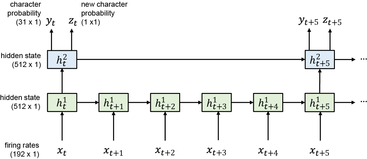
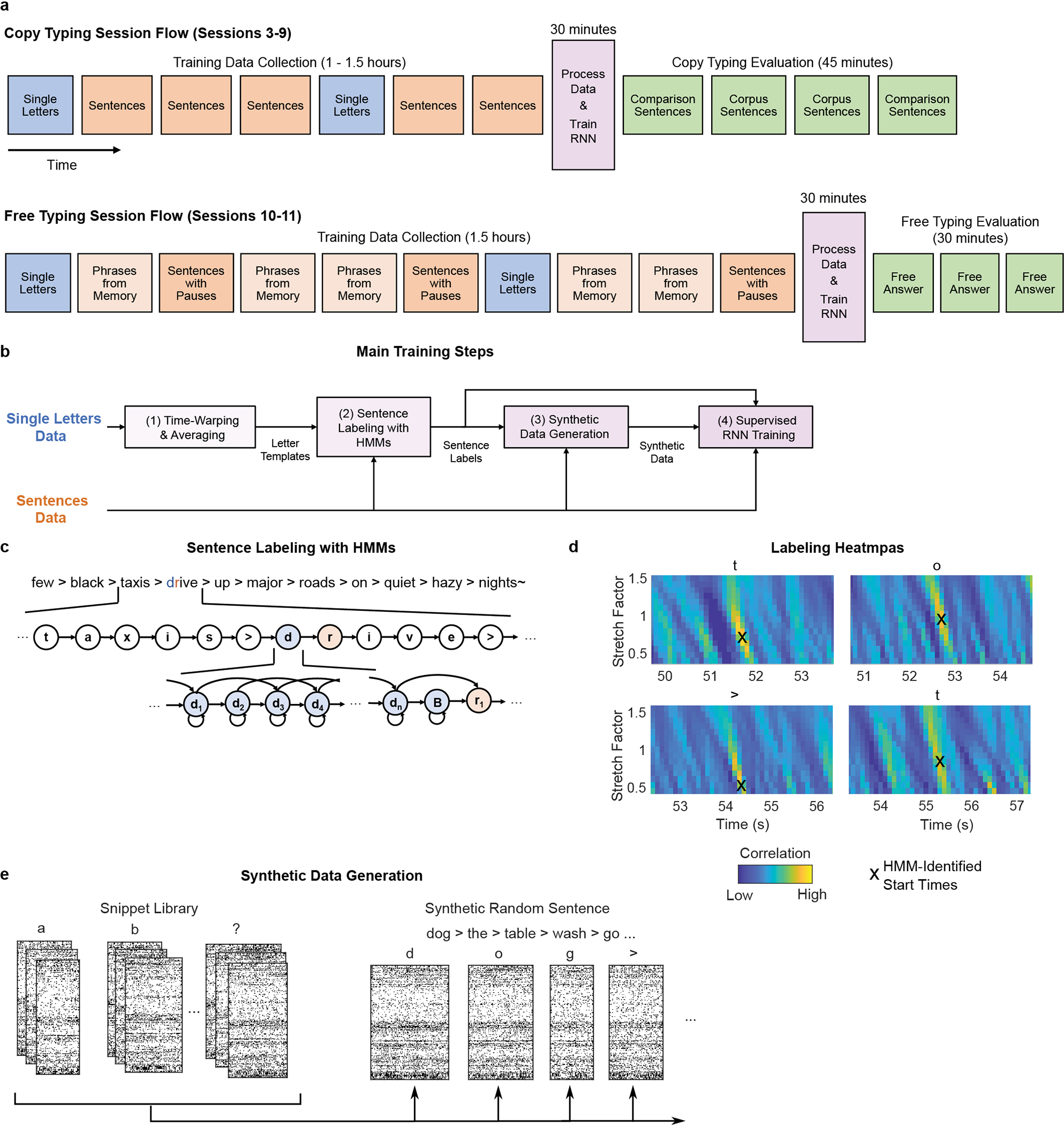
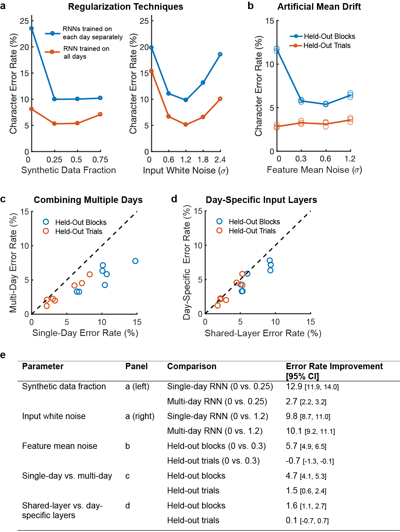
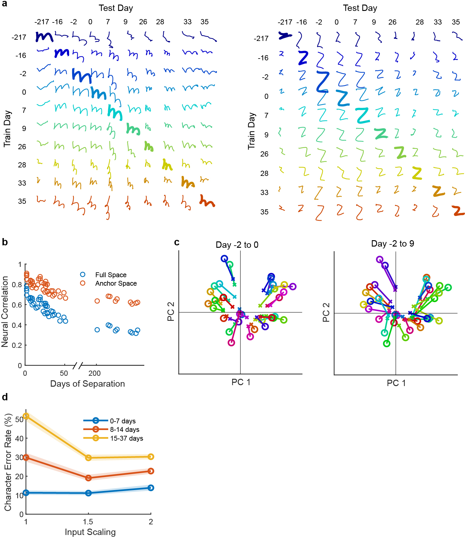
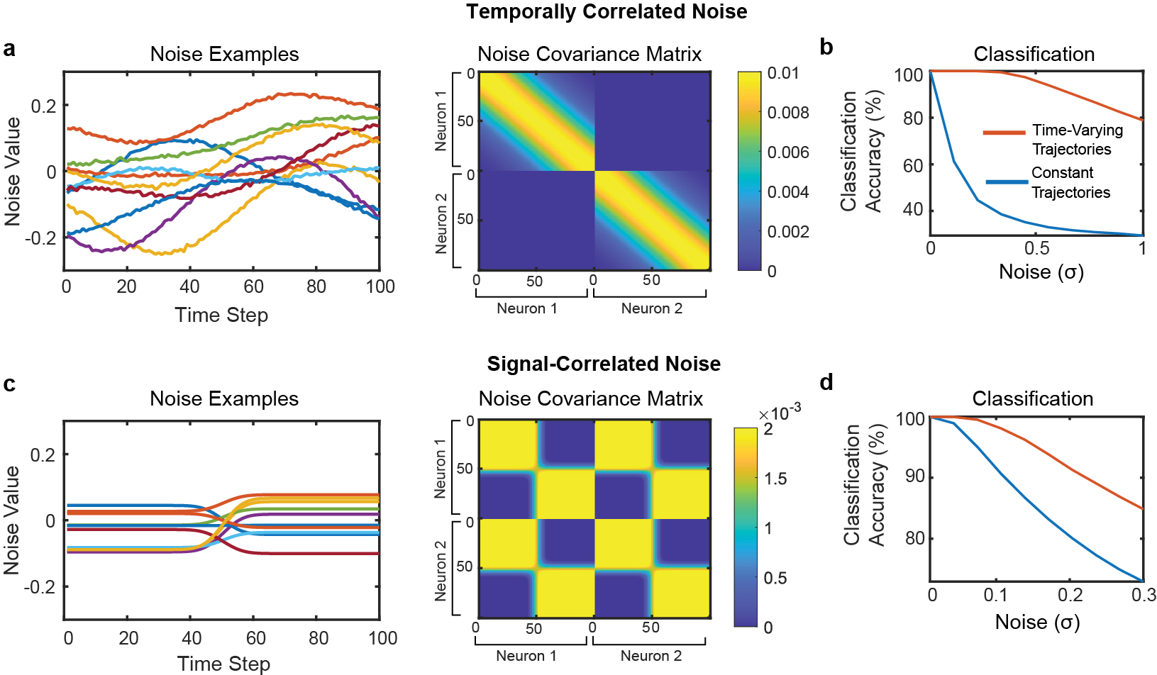
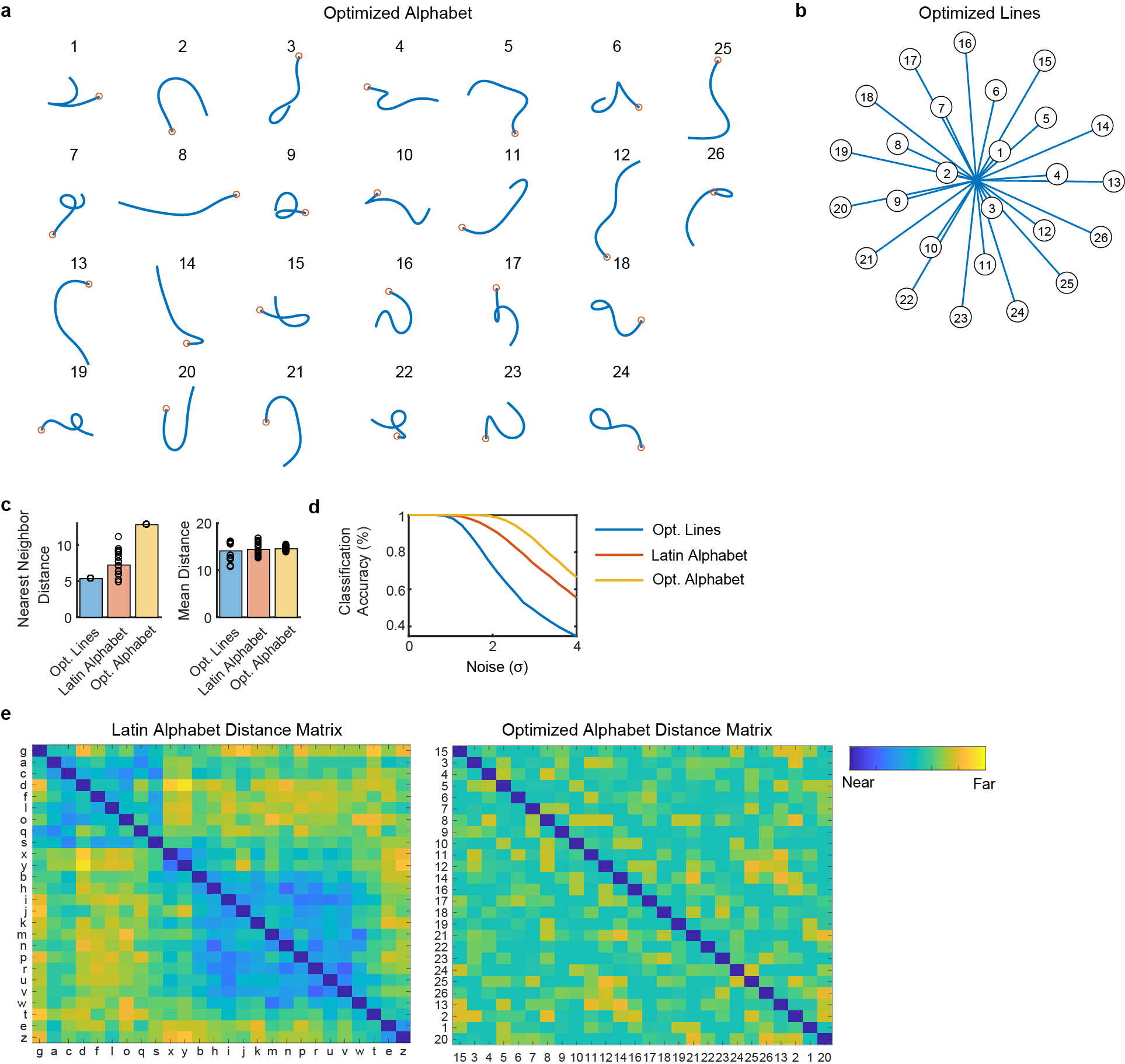
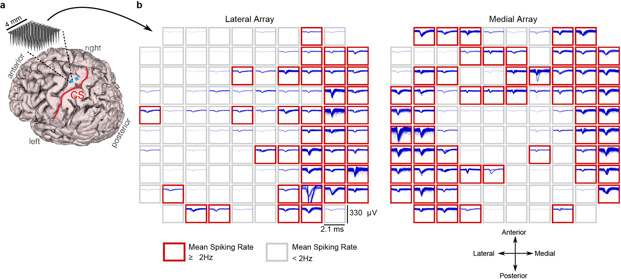
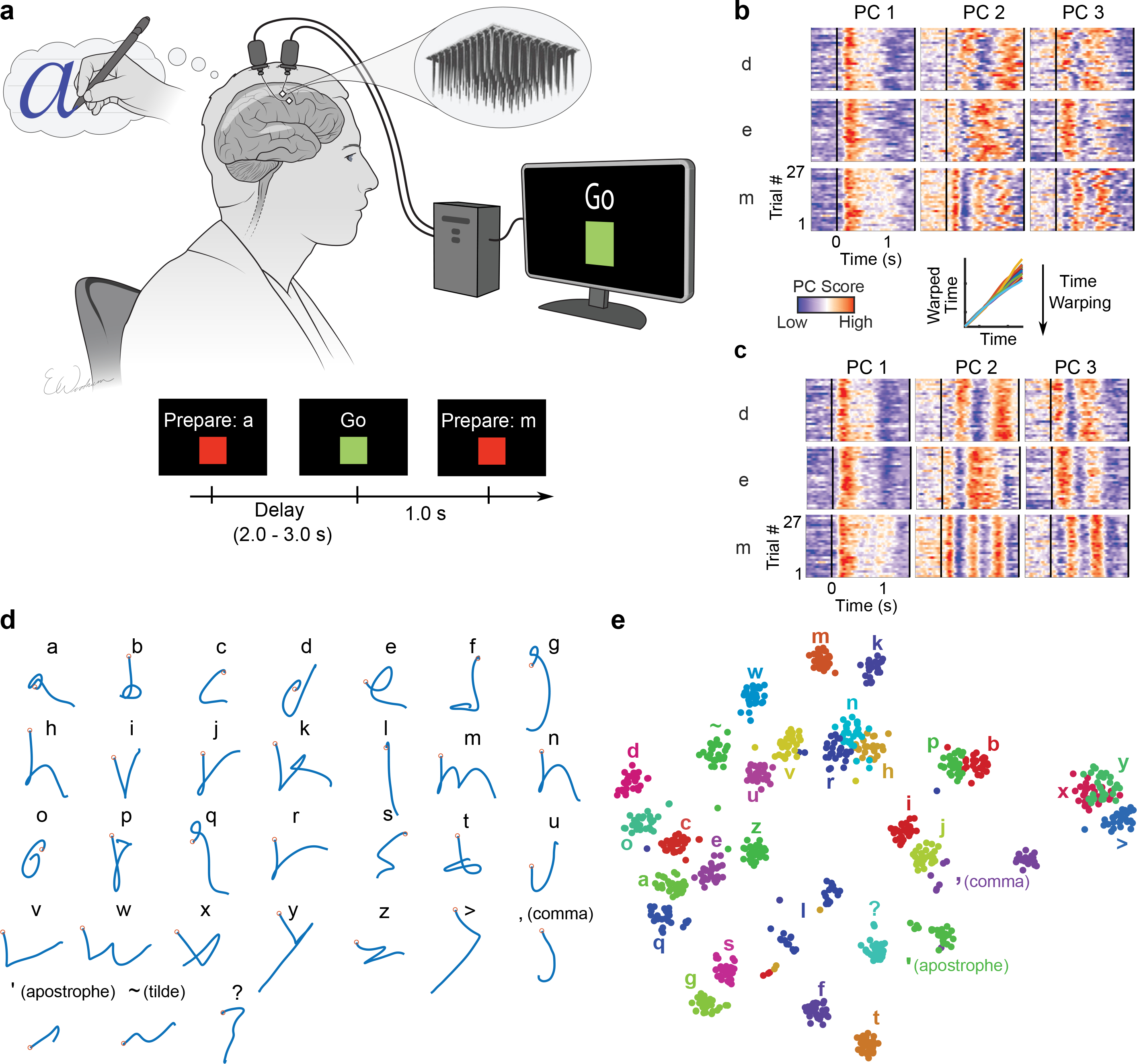
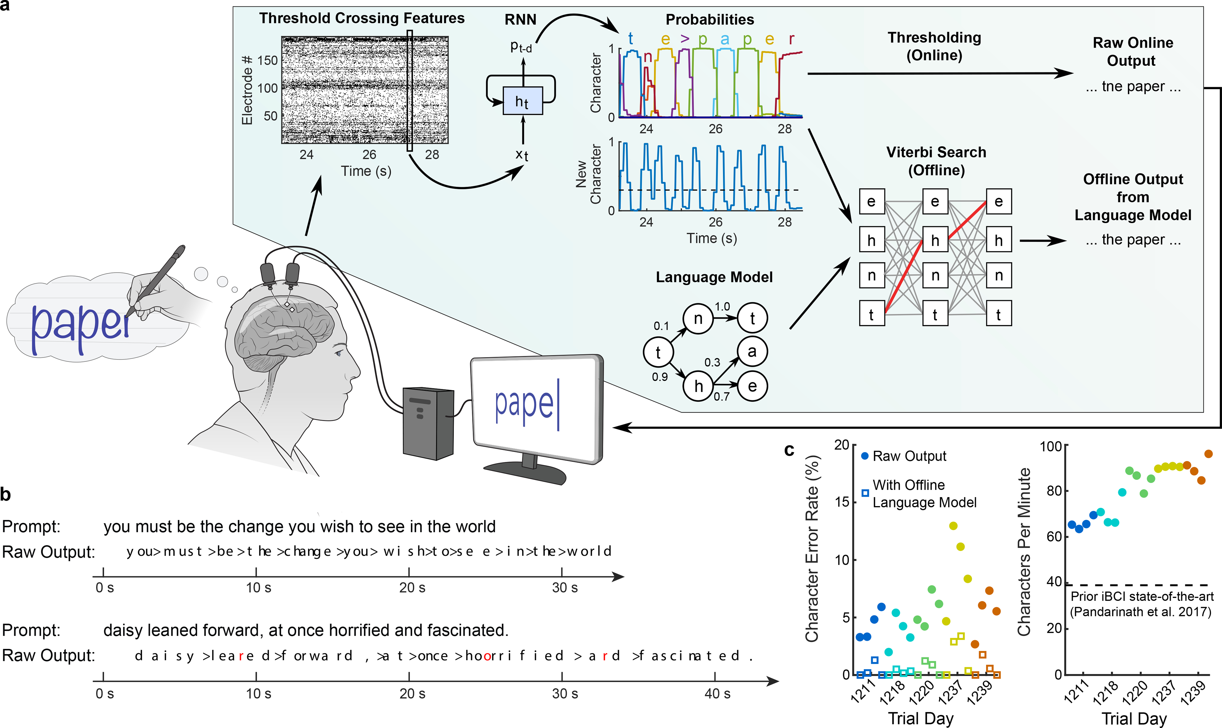
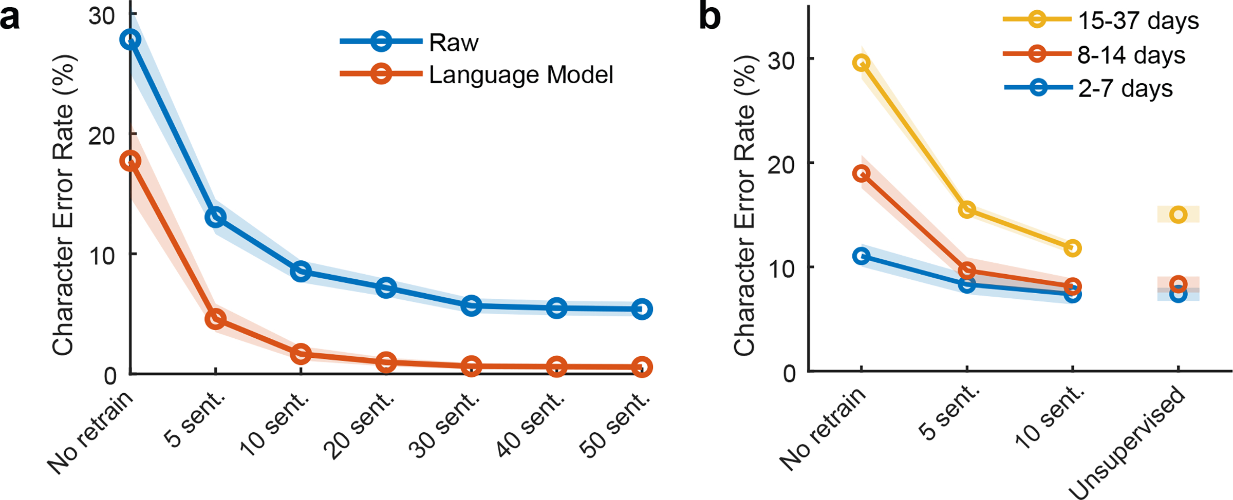
Brain-computer interfaces (BCIs) can restore communication to people who have lost the ability to move or speak. So far, a major focus of BCI research has been on restoring gross motor skills, such as reaching and grasping^1-5 or point-and-click typing with a computer cursor^6,7. However, rapid sequences of highly dexterous behaviours, such as handwriting or touch typing, might enable faster rates of communication. Here we developed an intracortical BCI that decodes attempted handwriting movements from neural activity in the motor cortex and translates it to text in real time, using a recurrent neural network decoding approach. With this BCI, our study participant, whose hand was paralysed from spinal cord injury, achieved typing speeds of 90 characters per minute with 94.1% raw accuracy online, and greater than 99% accuracy offline with a general-purpose autocorrect. To our knowledge, these typing speeds exceed those reported for any other BCI, and are comparable to typical smartphone typing speeds of individuals in the age group of our participant (115 characters per minute)⁸. Finally, theoretical considerations explain why temporally complex movements, such as handwriting, may be fundamentally easier to decode than point-to-point movements. Our results open a new approach for BCIs and demonstrate the feasibility of accurately decoding rapid, dexterous movements years after paralysis.

Extended Data Fig. 1:. Diagram of the RNN architecture.

We used a two-layer gated recurrent unit (GRU) recurrent neural network architecture to convert sequences of neural firing rate vectors x_t (which were temporally smoothed and binned at 20 ms) into sequences of character probability vectors y_t and ‘new character’ probability scalars z_t. The y_t vectors describe the probability of each character being written at that moment in time, and the z_t scalars go high whenever the RNN detects that T5 is beginning to write any new character. Note that the top RNN layer runs at a slower frequency than the bottom layer, which we found improved the speed of training by making it easier to hold information in memory for long time periods. Thus, the RNN outputs are updated only once every 100 ms.

Extended Data Fig. 2:. Overview of RNN training methods.

a, Diagram of the session flow for copy typing and free typing sessions (each rectangle corresponds to one block of data). First, single letter and sentences training data is collected (blue and red blocks). Next, the RNN is trained using the newly collected data plus all previous days’ data (purple block). Finally, the RNN is held fixed and evaluated (green blocks). b, Diagram of the data processing and RNN training process (purple block in a). First, the single letter data is time-warped and averaged to create spatiotemporal templates of neural activity for each character. These templates are used to initialize the hidden Markov models (HMMs) for sentence labeling. After labeling, the observed data is cut apart and rearranged into new sequences of characters to make synthetic sentences. Finally, the synthetic sentences are combined with the real sentences to train the RNN. c, Diagram of a forced-alignment HMM used to label the sentence “few black taxis drive up major roads on quiet hazy nights”. The HMM states correspond to the sequence of characters in the sentence. d, The label quality can be verified with cross-correlation heatmaps made by correlating the single character neural templates with the real data. The HMM-identified character start times form clear hotspots on the heatmaps. Note that these heatmaps are depicted only to qualitatively show label quality and aren’t used for training (only the character start times are needed to generate the targets for RNN training). e, To generate new synthetic sentences, the neural data corresponding to each labeled character in the real data is cut out of the data stream and put into a snippet library. These snippets are then pulled from the library at random, stretched/compressed in time by up to 30% (to add more artificial timing variability), and combined into new sentences.

Extended Data Fig. 3:. The effect of key RNN parameters on performance.

a, Training with synthetic data (left) and artificial white noise added to the inputs (right) were both essential for high performance. Data are shown from a grid search over both parameters, and lines show performance at the best value for the other parameter. Results indicate that both parameters are needed for high performance, even when the other is at the best value. Using synthetic data is more important when the dataset size is highly limited, as is the case when training on only a single day of data (blue line). Note that the inputs given to the RNN were z-scored, so the input white noise is in units of standard deviations of the input features. b, Artificial noise added to the feature means (random offsets and slow changes in the baseline firing rate) greatly improves the RNN’s ability to generalize to new blocks of data that occur later in the session, but does not help the RNN to generalize to new trials within blocks of data that it was already trained on. This is because feature means change slowly over time. For each parameter setting, three separate RNNs were trained (circles); results show low variability across RNN training runs. c, Training an RNN with all of the datasets combined improves performance relative to training on each day separately. Each circle shows the performance on one of seven days. d, Using separate input layers for each day is better than using a single layer across all days. e, Improvements in character error rates are summarized for each parameter. 95% confidence intervals were computed with bootstrap resampling of single trials (N=10,000). As shown in the table, all parameters show a statistically significant improvement for at least one condition (confidence intervals do not intersect zero).

Extended Data Fig. 4:. Changes in neural recordings across days.

a, To visualize how much the neural recordings changed across time, decoded pen tip trajectories were plotted for two example letters (“m” and “z”) for all ten days of data (columns), using decoders trained on all other days (rows). Each session is labeled according to the number of days passed relative to Dec. 9, 2019 (day #4). Results show that although neural activity patterns clearly change over time, their essential structure is largely conserved (since decoders trained on past days transfer readily to future days). b, The correlation (Pearson’s r) between each session’s neural activity patterns was computed for each pair of sessions and plotted as a function of the number of days separating each pair. Blue circles show the correlation computed in the full neural space (all 192 electrodes) while red circles show the correlation in the “anchor” space (top 10 principal components of the earlier session). High values indicate a high similarity in how characters are neurally encoded across days. The fact that correlations are higher in the anchor space suggests that the structure of the neural patterns stays largely the same as it slowly rotates into a new space, causing shrinkage in the original space but little change in structure. c, A visualization of how each character’s neural representation changes over time, as viewed through the top two PCs of the original “anchor” space. Each “o” represents the neural activity pattern for a single character, and each “x” shows that same character on a later day (lines connect matching characters). The left panel shows a pair of sessions with only two days between them (“Day −2 to 0”), while the right panel shows a pair of sessions with 11 days between them (“Day −2 to 9”). The relative positioning of the neural patterns remains similar across days, but most conditions shrink noticeably towards the origin. This is consistent with the neural representations slowly rotating out of the original space into a new space, and suggests that scaling-up the input features may help a decoder to transfer more accurately to a future session (by counteracting this shrinkage effect). d, Similar to Fig. 3b, copy typing data from eight sessions was used to assess offline whether scaling-up the decoder inputs improves performance when evaluating the decoder on a future session (when no decoder retraining is employed). All session pairs (X, Y) were considered. Decoders were first initialized using all data from session X and earlier, then evaluated on session Y under different input scaling factors (e.g., an input scale of 1.5 means that input features were scaled up by 50%). Lines indicate the average raw character error rate and shaded regions show 95% CIs. Results show that when long periods of time pass between sessions, input-scaling improves performance. We therefore used an input scaling factor of 1.5 when assessing decoder performance in the “no retraining” conditions of Fig. 3.

Extended Data Fig. 5:. Effect of correlated noise on the toy model of temporal dimensionality (see ^{Supplemental Note 1} for a detailed interpretation of this figure).

a, Example noise vectors and covariance matrix for temporally correlated noise. On the left, example noise vectors are plotted (each line depicts a single example). Noise vectors are shown for all 100 time steps of neuron 1. On the right, the covariance matrix used to generate temporally correlated noise is plotted (dimensions = 200 × 200). The first 100 time steps describe neuron 1’s noise and the last 100 time steps describe neuron 2’s noise. The diagonal band creates noise that is temporally correlated within each simulated neuron (but the two neurons are uncorrelated with each other). b, Classification accuracy when using a maximum likelihood classifier to classify between all four possible trajectories in the presence of temporally correlated noise. Even in the presence of temporally correlated noise, the time-varying trajectories are still much easier to classify. c, Example noise vectors and noise covariance matrix for noise that is correlated with the signal (i.e., noise that is concentrated only in spatiotemporal dimensions that span the class means). Unlike the temporally correlated noise, this covariance matrix generates spatiotemporal noise that has correlations between time steps and neurons. d, Classification accuracy in the presence of signal-correlated noise. Again, time-varying trajectories are easier to classify than constant trajectories.

Extended Data Fig. 6:. An artificial alphabet optimized to maximize neural decodability.

(A) Using the principle of maximizing the nearest neighbor distance, we optimized for a set of pen trajectories that are theoretically easier to classify than the Latin alphabet (using standard assumptions of linear neural tuning to pen tip velocity). (B) For comparison, we also optimized a set of 26 straight lines that maximize the nearest neighbor distance. (C) Pairwise Euclidean distances between pen tip trajectories were computed for each set, revealing a larger nearest neighbor distance (but not mean distance) for the optimized alphabet as compared to the Latin alphabet. Each circle represents a single movement and bar heights show the mean. (D) Simulated classification accuracy as a function of the amount of artificial noise added. Results confirm that the optimized alphabet is indeed easier to classify than the Latin alphabet, and that the Latin alphabet is much easier to classify than straight lines, even when the lines have been optimized. (E) Distance matrices for the Latin alphabet and optimized alphabets show the pairwise Euclidean distances between the pen trajectories. The distance matrices were sorted into 7 clusters using single-linkage hierarchical clustering. The distance matrix for the optimized alphabet has no apparent structure; in contrast, the Latin alphabet has two large clusters of similar letters (letters that begin with a counter-clockwise curl, and letters that begin with a down stroke).

Extended Data Fig. 7:. Example spiking activity recorded from each microelectrode array.

(A) Participant T5’s MRI-derived brain anatomy. Microelectrode array locations (blue squares) were determined by co-registration of postoperative CT images with preoperative MRI images. (B) Example spike waveforms detected during a ten second time window are plotted for each electrode (data were recorded on post-implant day 1218). Each rectangular panel corresponds to a single electrode and each blue trace is a single spike waveform (2.1 millisecond duration). Spiking events were detected using a −4.5 RMS threshold, thereby excluding almost all background activity. Electrodes with a mean threshold crossing rate ≥ 2 Hz were considered to have ‘spiking activity’ and are outlined in red (note that this is a conservative estimate that is meant to include only spiking activity that could be from single neurons, as opposed to multiunit ‘hash’). Results show that many electrodes still record large spiking waveforms that are well above the noise floor (the y-axis of each panel spans 330 μV, while the background activity has an average RMS value of only 6.4 μV). On this day, 92 electrodes out of 192 had a threshold crossing rate ≥ 2 Hz.

Figure 1.. Neural representation of attempted handwriting.

a, To assess the neural representation of attempted handwriting, participant T5 attempted to handwrite each character one at a time, following the instructions given on a computer screen (lower panels depict what is shown on the screen, following the timeline). b, Neural activity in the top 3 principal components (PCs) is shown for three example letters (d, e and m) and 27 repetitions of each letter (‘trials’). The color scale was normalized within each panel separately for visualization. c, Time-warping the neural activity to remove trial-to-trial changes in writing speed reveals consistent patterns of activity unique to each letter. In the inset above C, example time-warping functions are shown for the letter ‘m’ and lie relatively close to the identity line (each trial’s warping function is plotted with a differently colored line). d, Decoded pen trajectories are shown for all 31 tested characters. Intended 2D pen tip velocity was linearly decoded from the neural activity using cross-validation (each character was held out), and decoder output was denoised by averaging across trials. Orange circles denote the start of the trajectory. e, A 2-dimensional visualization of the neural activity made using t-SNE. Each circle is a single trial (27 trials for each of 31 characters).

Figure 2.. Neural decoding of attempted handwriting in real-time.

a, Diagram of the decoding algorithm. First, the neural activity (multiunit threshold crossings) was temporally binned and smoothed on each electrode (20 ms bins). Then, a recurrent neural network (RNN) converted this neural population time series (x_t) into a probability time series (p_t-d) describing the likelihood of each character and the probability of any new character beginning. The RNN had a one second output delay (d), giving it time to observe each character fully before deciding its identity. Finally, the character probabilities were thresholded to produce “Raw Online Output” for real-time use (when the ‘new character’ probability crossed a threshold at time t, the most likely character at time t+0.3s was emitted and shown on the screen). In an offline retrospective analysis, the character probabilities were combined with a large-vocabulary language model to decode the most likely text that the participant wrote (using a custom 50,000-word bigram model). b, Two real-time example trials are shown, demonstrating the RNN’s ability to decode readily understandable text on sentences it was never trained on. Errors are highlighted in red and spaces are denoted with “>”. c, Error rates (edit distances) and typing speeds are shown for five days, with four blocks of 7–10 sentences each (each block is indicated with a single circle and colored according to the trial day). The speed is more than double that of the next fastest intracortical BCI.

Figure 3.. Performance remains high when daily decoder retraining is shortened (or unsupervised).

a, To account for neural activity changes that accrue over time, we retrained our handwriting decoder each day before evaluating it. Here, we simulated offline how decoding performance would have changed if less than the original 50 calibration sentences were used. Lines show the mean error rate across all data and shaded regions indicate 95% CIs. b, Copy typing data from eight sessions were used to assess whether less calibration data are required if sessions occur closer in time. All session pairs (X, Y) were considered. Decoders were first initialized using training data from session X and earlier, and then evaluated on session Y under different retraining methods (no retraining, retraining with limited calibration data, or unsupervised retraining). Lines show the average raw error rate and shaded regions indicate 95% CIs.

Figure 4.. Increased temporal variety can make movements easier to decode.

a, We analyzed the spatiotemporal patterns of neural activity corresponding to 16 handwritten characters (1 second in duration) vs. 16 handwritten straight-line movements (0.6 seconds in duration). b, Spatiotemporal neural patterns were found by averaging over all trials for a given movement (after time-warping to align the trials in time). Neural activity was resampled to equalize the duration of each set of movements, resulting in a 192 × 100 matrix for each movement (192 electrodes and 100 time steps). c, Pairwise Euclidean distances between neural patterns were computed for each set, revealing larger nearest neighbor distances (but not mean distances) for characters. Each circle represents a single movement and bar heights show the mean. d, Larger nearest neighbor distances made the characters easier to classify than straight lines. The noise is in units of standard deviations and matches the scale of the distances in c. e, The spatial dimensionality was similar for characters and straight lines, but the temporal dimensionality was more than twice as high for characters, suggesting that more temporal variety underlies the increased nearest neighbor distances and better classification performance. Error bars show the 95% CI. Dimensionality was quantified using the participation ratio. f-h, A toy example to give intuition for how increased temporal dimensionality can make neural trajectories more separable. Four neural trajectories are depicted (N1 and N2 are two hypothetical neurons whose activity is constrained to a single spatial dimension, the unity diagonal). Allowing the trajectories to vary in time by adding one bend (increasing the temporal dimensionality from 1 to 2) enables larger nearest neighbor distances (g) and better classification (h).

References

1. Hochberg LR et al. Reach and grasp by people with tetraplegia using a neurally controlled robotic arm. Nature 485, 372–375 (2012). - PMC - PubMed
1. Collinger JL et al. High-performance neuroprosthetic control by an individual with tetraplegia. The Lancet 381, 557–564 (2013). - PMC - PubMed
1. Aflalo T et al. Decoding motor imagery from the posterior parietal cortex of a tetraplegic human. Science 348, 906–910 (2015). - PMC - PubMed
1. Bouton CE et al. Restoring cortical control of functional movement in a human with quadriplegia. Nature 533, 247–250 (2016). - PubMed
1. Ajiboye AB et al. Restoration of reaching and grasping movements through brain-controlled muscle stimulation in a person with tetraplegia: a proof-of-concept demonstration. The Lancet 389, 1821–1830 (2017). - PMC - PubMed
Publication types