Processing single-cell RNA-seq data for dimension reduction-based analyses using open-source tools

Abstract

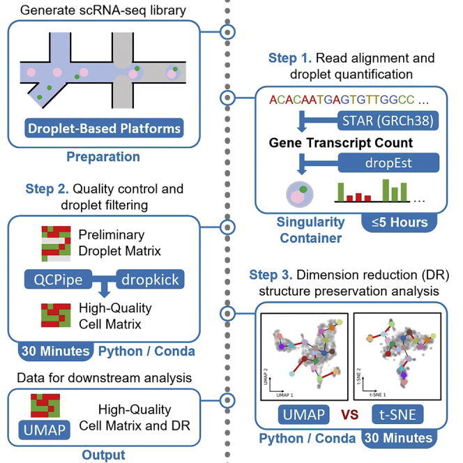
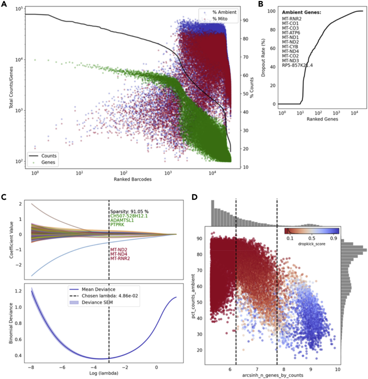
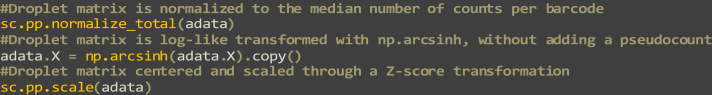
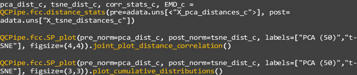
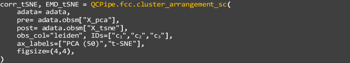
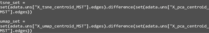
Single-cell RNA sequencing data require several processing procedures to arrive at interpretable results. While commercial platforms can serve as "one-stop shops" for data analysis, they relinquish the flexibility required for customized analyses and are often inflexible between experimental systems. For instance, there is no universal solution for the discrimination of informative or uninformative encapsulated cellular material; thus, pipeline flexibility takes priority. Here, we demonstrate a full data analysis pipeline, constructed modularly from open-source software, including tools that we have contributed. For complete details on the use and execution of this protocol, please refer to Petukhov et al. (2018), Heiser et al. (2020), and Heiser and Lau (2020).

Keywords: Bioinformatics; RNA-seq.

Graphical abstract

Figure 1

Inflection curve analysis (A and B) Inflection curve thresholding (A) for a high quality dataset with corresponding Total Counts to N Genes By Counts ratio plot on log scales (B). (C and D) Inflection curve thresholding (C) for a low quality dataset with corresponding Total Counts to N Genes By Counts ratio plot on log scales (D). Red arrows indicate inflection points (A and B), and red brackets indicate the ‘plateau’ motif in the Total Counts/N Genes By Counts plot.

Figure 2

Relative transcript diversity distribution analysis (Aa nd B) Relative transcript diversity histogram plot (A) for a high quality dataset with corresponding UMAP with highlighted selection (B). (C and D) Relative transcript diversity histogram plot (C) for a low quality dataset with corresponding UMAP with highlighted selection (D). Red arrows indicate bimodality and unimodality in (A and C), respectively, for the distributions of transcript diversity.

Figure 3

Heuristic cluster selection criteria (A) Marker gene UMAP overlays, with scale bars denoting the normalized and transformed values. (B) Leiden cluster labels derived through the Leiden community detection algorithm at a resolution of 2. (C) UMAP visualization of the selected clusters, being 9, 11, 16, 21, and 22.

Figure 4

Automated droplet filtering with dropkick (A) Profile of total counts (black trace) and genes (green points) detected per ranked barcode for human colonic mucosa sample. Percentage of mitochondrial (red) and ambient (blue) reads for each barcode included to denote quality along total counts profile. (B) Ranked gene dropout rates. Ambient genes identified by dropkick are used to calculate percent ambient counts in A. (C) Plot of coefficient values for 2,000 highly variable genes (top) and mean binomial deviance ± SEM (bottom) for model cross-validation along the lambda regularization path defined by dropkick. Top and bottom three coefficients are shown, in axis order, along with total model sparsity (top). Chosen lambda value shown as dashed vertical line. (D) Plot of percent ambient counts versus arcsinh-transformed genes detected per barcode, with histogram distributions plotted on margins. Initial dropkick training thresholds shown as dashed vertical lines. Each point (barcode) is colored by its final cell probability after model fitting.

Figure 5

PCA of human colonic mucosa dataset with PAGA graph (A) Top and bottom 15 gene loadings for the first three PCs. (B) Proportion of total explained variance for each of the top 30 PCs. (C) First two PCs plotted with Leiden cluster overlay. (D) PAGA graph constructed from k-nearest neighbors (kNN) in 50-component PCA space (k = 46), describing relationships between Leiden clusters.

Figure 6

Global comparison of two-dimensional embeddings of human colonic mucosa dataset (A) t-SNE embedding seeded with 50-component PCA, plotted with overlay of Leiden clustering. (B) UMAP embedding seeded with 50-component PCA and initialized with PAGA coordinates, plotted with overlay of Leiden clustering. (C) Global structural preservation correlation plot comparing t-SNE coordinates (latent space) to 50-component PCA (native space). (D) Same as in (C), comparing UMAP coordinates (latent space) to 50-component PCA (native space). Indicated with red arrows in (C) and (D) are latent space distance distributions which differ between t-SNE and UMAP. (E) Top four differentially expressed genes for each Leiden cluster, with signatures for clusters 3, 4, 8, and 11 highlighted.

Figure 7

Local and organizational structure preservation analysis for human colonic mucosa dataset (A) t-SNE embedding highlighting tuft cell cluster. (B) Local structure preservation correlation plot for tuft cell cluster, comparing t-SNE coordinates (latent space) to 50-component PCA (native space). (C) t-SNE embedding highlighting secretory lineage from stem cells (cluster 3) to goblet cells (cluster 8) and mature goblet cells (clusters 4 and 12). (D) Structure preservation correlation plot showing distances between stem and mature cell lineage clusters. Indicated with red arrows in (B and G) and (D and I) are latent space distance distributions which differ between t-SNE and UMAP. (E) t-SNE embedding with minimum spanning tree (MST) drawn between Leiden cluster centroids. Red edges represent those not present in native (PCA) space. (F–J) Same as in (A–E), for UMAP embedding.

References

1. Van der Auwera G.A., Carneiro M.O., Hartl C., Poplin R., del Angel G., Levy-Moonshine A., Jordan T., Shakir K., Roazen D., Thibault J. From fastQ data to high-confidence variant calls: The genome analysis toolkit best practices pipeline. Curr. Protoc. Bioinformatics. 2013;43:11.10.1–11.10.33. - PMC - PubMed
1. Barnett D.W., Garrison E.K., Quinlan A.R., Strömberg M.P., Marth G.T. BamTools: a C++ API and toolkit for analyzing and managing BAM files. Bioinformatics. 2011;27:1691–1692. - PMC - PubMed
1. Bates D., Eddelbuettel D. Fast and elegant numerical linear algebra using the rcppeigen package. J. Stat. Softw. 2013;52:1–24. - PubMed
1. Chen B., Herring C.A., Lau K.S. pyNVR: investigating factors affecting feature selection from scRNA-seq data for lineage reconstruction. Bioinformatics. 2018;35:2335–2337. - PMC - PubMed
1. Csardi G., Nepusz T. The igraph software package for complex network research. InterJ. Comp. Syst. 2006:1695.
Publication types
LinkOut - more resources