. 2021 May 13;12(1):2785.
doi: 10.1038/s41467-021-22856-z.

Cellular connectomes as arbiters of local circuit models in the cerebral cortex

Affiliations

Cellular connectomes as arbiters of local circuit models in the cerebral cortex

Emmanuel Klinger et al. Nat Commun. .

Abstract

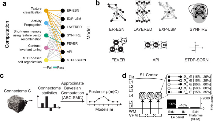
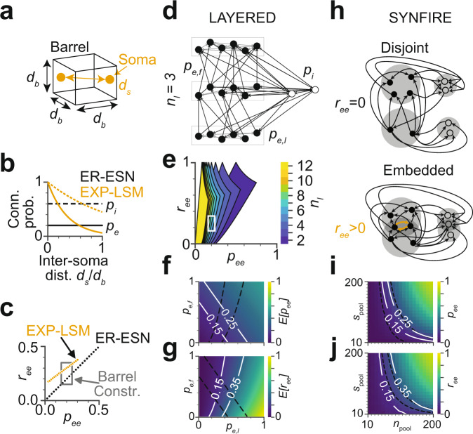
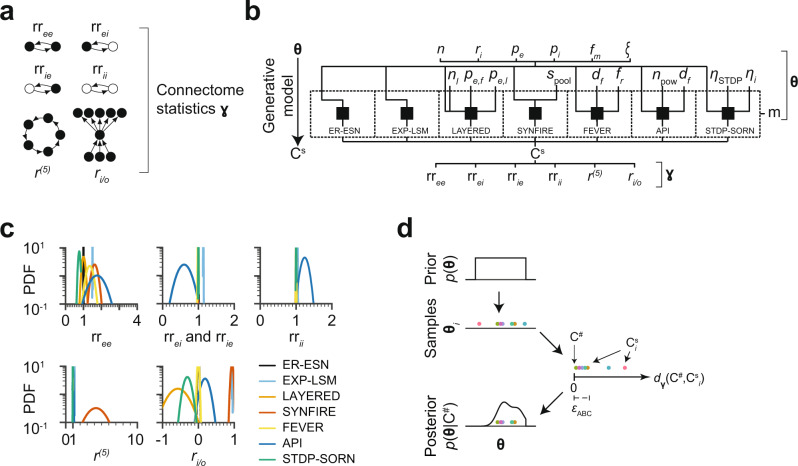
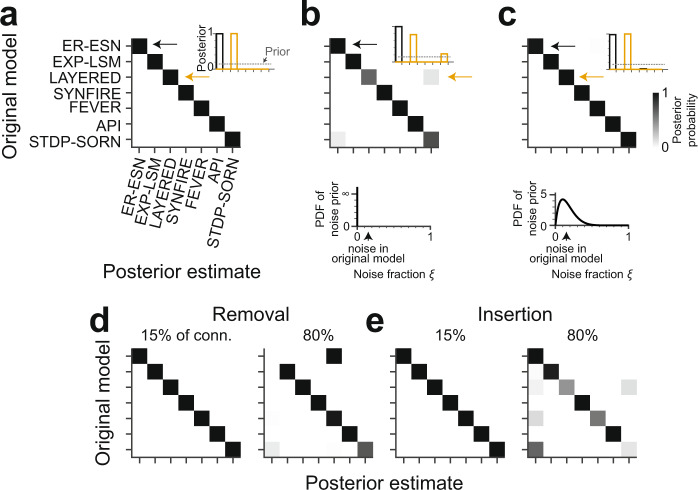
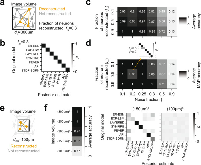
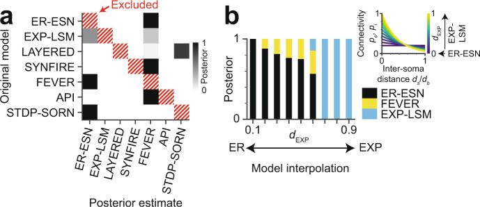
With the availability of cellular-resolution connectivity maps, connectomes, from the mammalian nervous system, it is in question how informative such massive connectomic data can be for the distinction of local circuit models in the mammalian cerebral cortex. Here, we investigated whether cellular-resolution connectomic data can in principle allow model discrimination for local circuit modules in layer 4 of mouse primary somatosensory cortex. We used approximate Bayesian model selection based on a set of simple connectome statistics to compute the posterior probability over proposed models given a to-be-measured connectome. We find that the distinction of the investigated local cortical models is faithfully possible based on purely structural connectomic data with an accuracy of more than 90%, and that such distinction is stable against substantial errors in the connectome measurement. Furthermore, mapping a fraction of only 10% of the local connectome is sufficient for connectome-based model distinction under realistic experimental constraints. Together, these results show for a concrete local circuit example that connectomic data allows model selection in the cerebral cortex and define the experimental strategy for obtaining such connectomic data.


Conflict of interest statement

The authors declare no competing interests

Figures

Fig. 1
Fig. 1. Relationship between models and possible computations in cortical circuits, and proposed strategy for connectomic model distinction in local circuit modules of the cerebral cortex.
a Relationship between computations suggested for local cortical circuits (left) and possible circuit-level implementations (right). Colored lines indicate successful performance in the tested computation; gray lines indicate failure to perform the computation (see Supplementary Fig. 1 for details). b Enumeration of candidate models possibly implemented in a barrel-circuit module. See text for details. c Flowchart of connectomic model selection approach to obtain the posterior p (m|C) over hypothesized models m given a connectome C. ABC-SMC: approximate Bayesian computation using sequential Monte–Carlo sampling. d Sketch of mouse primary somatosensory cortex with presumed circuit modules (“barrels”) in cortical input layer 4 (L4). Currently known constraints of pairwise connectivity and cell prevalence of excitatory (ExN) and inhibitory (IN) neurons (pee: pairwise excitatory-excitatory connectivity–,, pei: pairwise excitatory-inhibitory connectivity,, pii: pairwise inhibitory-inhibitory connectivity,, pie: pairwise inhibitory-excitatory connectivity,,, ree: pairwise excitatory-excitatory reciprocity,,).
Fig. 2
Fig. 2. Compliance of candidate models with the so-far experimentally determined pairwise barrel circuit constraints in L4 (see Fig. 1d).
a Illustration of a simplified cortical barrel of width db and somata with inter soma distance ds. b Pairwise excitatory and inhibitory connection probabilities pe and pi are constant over inter soma distance ds in the Erdős–Rényi echo state network (ER-ESN) and decay in the exponentially decaying connectivity - liquid state machine model (EXP-LSM). c Possible pairwise excitatory-excitatory connectivity pee and excitatory-excitatory reciprocity ree in the ER-ESN and EXP-LSM model satisfy the so-far determined barrel constraints (box). dg Layered model: d example network with three layers (nl=3), excitatory forward (between-layer) connectivity pe,f, excitatory lateral (within-layer) connectivity pe,l and inhibitory connectivity pi. e Range of pee and ree in the LAYERED model for varying number of layers nl (white box: barrel constraints as in c). f, g Expected excitatory pairwise connectivity Epee and reciprocity Eree as function of pe,l and pe,f for nl=3. Isolines indicate barrel constraints, model parameters in compliance with these constraints: area between intersecting isolines. Note that constraints are fulfilled only for within-layer connectivity pe,l>0, refuting a strictly feedforward network. hj Embedded synfire chain model (SYNFIRE). h Two subsequent synfire pools in the disjoint (top) and embedded (bottom) synfire chain. Since intra-pool connectivity pe,l is strictly zero, reciprocal connections do not exist in the disjoint case (ree=0) but in the embedded configuration. i, j Pairwise excitatory connectivity pee and pairwise excitatory reciprocity ree as function of the number of pools npool and the pool size spool for a SYNFIRE network with N=2000 neurons. Respective barrel constraints (white and dashed line). See Supplementary Fig. 2 for analogous analysis of FEVER, API, and STDP-SORN models.
Fig. 3
Fig. 3. Connectome statistics and generative models for approximate Bayesian inference.
a Connectome statistics γ used for model distinction: relative excitatory-excitatory reciprocity rree, relative excitatory-inhibitory reciprocity rrei, relative inhibitory-excitatory reciprocity rrie, relative inhibitory-inhibitory reciprocity rrii, relative cycles of length 5, r(5), and in-out degree correlation of excitatory neurons ri/o. b Generative model for Bayesian inference: shared set of parameters (top: number of neurons n, fraction of inhibitory neurons ri, excitatory connectivity pe, inhibitory connectivity pi, fractional connectome measurement fm, noise ξ) and model-specific parameters (middle: model choice m, number of layers nl, excitatory forward connectivity pe,f, excitatory lateral connectivity pe,l, pool size spool, STDP learning rate ηSTDP, intrinsic learning rate ηi, feature space dimension df, feverization ratio fr, selectivity npow, see Supplementary Fig. 4), generated sampled connectome Cs described by the summary statistics γ=(rree,rrei,rrie,rrii,r5,ri/o). c Gaussian fits of probability density functions (PDFs) of the connectome statistics γ (a) for all models (see Fig. 1b). d Sketch of ABC-SMC procedure: given a measured connectome C#, parameters θi (colored dots) are sampled from the prior p(θ). Each θi generates a connectome Cis that has a certain distance dγC#,Cis to C# in the space defined by the connectome statistics γ (a). If this distance is below a threshold ϵABC, the associated parameters θi are added as mass to the posterior distribution pθC#, and are rejected otherwise.
Fig. 4
Fig. 4. Identification of models using Bayesian model selection under ideal and noisy connectome measurements.
a Confusion matrix reporting the posteriors over models given example connectomes. Example connectomes were sampled from each model class (rows; Fig. 3b) and then exposed to the ABC-SMC method (Fig. 3d) using only the connectome statistics (Fig. 3a). Note that all model classes are uniquely identified from the connectomes (inset: average posteriors for ER-ESN and LAYERED connectomes, respectively; n = 3 repetitions). b Posteriors over models given example connectomes to which a random noise of 15% (inset, dashed line) was added before applying the ABC-SMC method. The generative model (Fig. 3b) was ignorant of this noise (n = 3 repetitions; bottom: noise prior pξ=δξ,0). c Same analysis as in b, this time including a noise prior into the generative model (n = 3 repetitions). Bottom: The noise prior was modeled as pξ=Beta(2, 10). Note that in most connectome measurements, the level of reconstruction errors is quantifiable, such that the noise can be rather faithfully incorporated into the noise prior (see text). Model identification is again accurate under these conditions (compare c and a). d Confusion matrix when simulating split errors in neuron reconstructions by randomly removing 15% (left) or 80% (right) of connections before ABC-SMC inference. e Confusion matrix when simulating merge errors in neuron reconstructions by insertion of additional 15% (left) and 80% (right) of the original number of connections into random locations in the connectome before ABC-SMC inference. d, e Noise prior during ABC-SMC inference was of the same type as the simulated reconstruction errors (n = 1 repetition; noise prior pξ=Beta(2, 10)). Color bar in c applies to all panels.
Fig. 5
Fig. 5. Model selection for partially measured and noisy connectomes.
a Fractional (incomplete) connectome measurement when reconstructing only a fraction fm of the neurons in a given circuit, thus obtaining a fraction fm2 of the complete connectome. b Effect of incomplete connectome measurement on model selection performance for fm = 0.3 (no noise; n = 1 repetition). Note that model selection is still faithfully possible. c, d Combined effects of noisy and incomplete connectome measurements on model selection accuracy reported as average posterior probability (c; n = 1 repetition per entry) and maximum-a-posteriori accuracy (d; n = 1 repetition per entry). Note that model selection is highly accurate down to 10% fractional connectome measurement at up to 25% noise, providing an experimental design for model distinction that is realistic under current connectome measurement techniques (see text). Model selection used a fixed pξ=Beta(2, 10) noise prior. More informative noise priors result in more accurate model selection (Supplementary Fig. 5b). e Effect of fractional dense circuit reconstruction: Locally dense connectomic reconstruction of the neurons and of their connections in a circuit subvolume. f Effect of partial imaging and dense reconstruction of the circuit subvolume on average model selection accuracy (left: n = 1 repetition per entry). Note that model selection based on dense reconstruction of a (150 μm)3 volume (12.5% of circuit volume) is substantially less accurate than model selection based on complete reconstructions of 10% in the complete circuit volume (see c). Right: Posterior distributions over models for image volumes of (150 μm)3 and (100 μm)3, respectively (n = 1 repetition, each).
Fig. 6
Fig. 6. Effect of incomplete hypothesis space and of model interpolation on Bayesian model selection.
a Confusion matrix reporting the posterior distribution when excluding the true model (hatched) from the set of tested model hypotheses (n = 1 repetition). Note that posterior probability is non-uniformly distributed and concentrated at plausibly similar models even when the true model is not part of the hypothesis space. b Posterior distributions for connectome models interpolated between ER-ESN and EXP-LSM (n = 1 repetition per bar). Inset: Space constant dEXP acts as interpolation parameter between ER-ESN (dEXP = 0) and EXP-LSM (dEXP = 1). Note that the transition between the two models is captured by the estimated model posterior, with an intermediate (non-dominant) confusion with the FEVER model.
Fig. 7
Fig. 7. Connectomic separability of recurrent neural network (RNNs) with similar initialization, but trained on different tasks.
a Overview of training process: RNNs were initially fully connected. Whenever task performance saturated during training, the weakest 10% of connections were pruned (†) to obtain a realistic level of sparsity. b Task performance (black) and network connectivity (gray) of a texture discrimination RNN during training. Ticks indicate the pruning of connections. Inset (*): Connection pruning causes a decrease in task performance, which is (partially) compensated by further training of the remaining connections. c Task performance as a function of network connectivity (p). Performance defined as: Accuracy (Texture discrimination RNNs, gray); 1 – mean squared error (Sequence memorization RNNs, magenta). Note that maximum observed performance was achieved in a wide connectivity regime including connectivity consistent with experimental data (pS1 = 24%; dashed line). Task performance started to decay after pruning at least 99.6% of connections. d Connectome statistics of RNNs over iterative training and pruning of connections (cf. Fig. 3a). e Distribution of connectome statistics at p = pS1 for RNNs and structural network models. Note that structural network models and structurally unconstrained RNNs exhibit comparable variance in connectome statistics (rree: 0.088 vs. 0.15 for API; rrei and rrie: 0.0019 vs. 0.026 for API; rrii: 9.35 × 10⁻⁷ vs. 8.17 × 10⁻³ for API; r(5): 1.54 vs. 1.51 for SYNFIRE; ri/o: 0.057 vs. 0.061 for LAYERED; cf. Fig. 3c). RNNs trained on different tasks did not differ significantly in terms of connectome statistics (rree: 1.48 ± 0.30 vs. 1.46 ± 0.29, p = 0.997; rrei and rrie: 1.00 ± 0.04 vs. 0.99 ± 0.01, p = 0.534; rrii: 1.01 ± 0.01 vs. 1.01 ± 0.00, p = 0.107; r(5): 2.28 ± 1.24 vs. 1.84 ± 0.80, p = 0.997; ri/o: 0.31 ± 0.24 vs. 0.49 ± 0.12, p = 0.534; mean ± std for n = 4 texture discrimination vs. sequence memorization RNNs, each; two-sided Kolmogorov-Smirnov test without correction for multiple comparisons). Boxes: center line is median; box limits are quartiles; whiskers are minimum and maximum; all data points shown. f Similarity of RNNs based on connectome statistics (lines) as connectivity approaches biologically plausible connectivity pS1 (circles and arrows, left) and for connectivity range from 100% to 0.04% (circles and arrows, right). Note that connectome statistics at ≤11% connectivity separate texture discrimination and sequence memorization RNNs into two clusters. g Distribution of connection strengths at p = pS1 for two RNNs trained on different tasks. h Connectome statistics of RNNs with pS1 connectivity when ignoring weak connections. i Separability of texture discrimination and sequence memorization RNNs with biologically plausible connectivity based on statistics derived from weighted connectome.

References

    1. Doyle DA, et al. The structure of the potassium channel: molecular basis of K+ conduction and selectivity. Science. 1998;280:69–77. doi: 10.1126/science.280.5360.69. - DOI - PubMed
    1. Nogales E. The development of cryo-EM into a mainstream structural biology technique. Nat. Methods. 2016;13:24–27. doi: 10.1038/nmeth.3694. - DOI - PMC - PubMed
    1. Bargmann CI, Marder E. From the connectome to brain function. Nat. Methods. 2013;10:483–490. doi: 10.1038/nmeth.2451. - DOI - PubMed
    1. Morgan JL, Lichtman JW. Why not connectomics? Nat. Methods. 2013;10:494–500. doi: 10.1038/nmeth.2480. - DOI - PMC - PubMed
    1. Denk W, Briggman KL, Helmstaedter M. Structural neurobiology: missing link to a mechanistic understanding of neural computation. Nat. Rev. Neurosci. 2012;13:351–358. doi: 10.1038/nrn3169. - DOI - PubMed

LinkOut - more resources