Hierarchical progressive learning of cell identities in single-cell data

Abstract

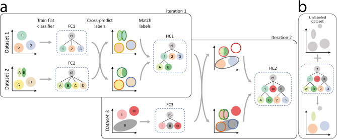
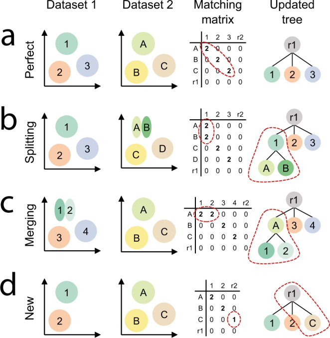
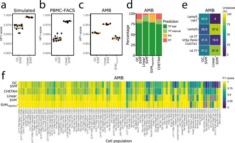
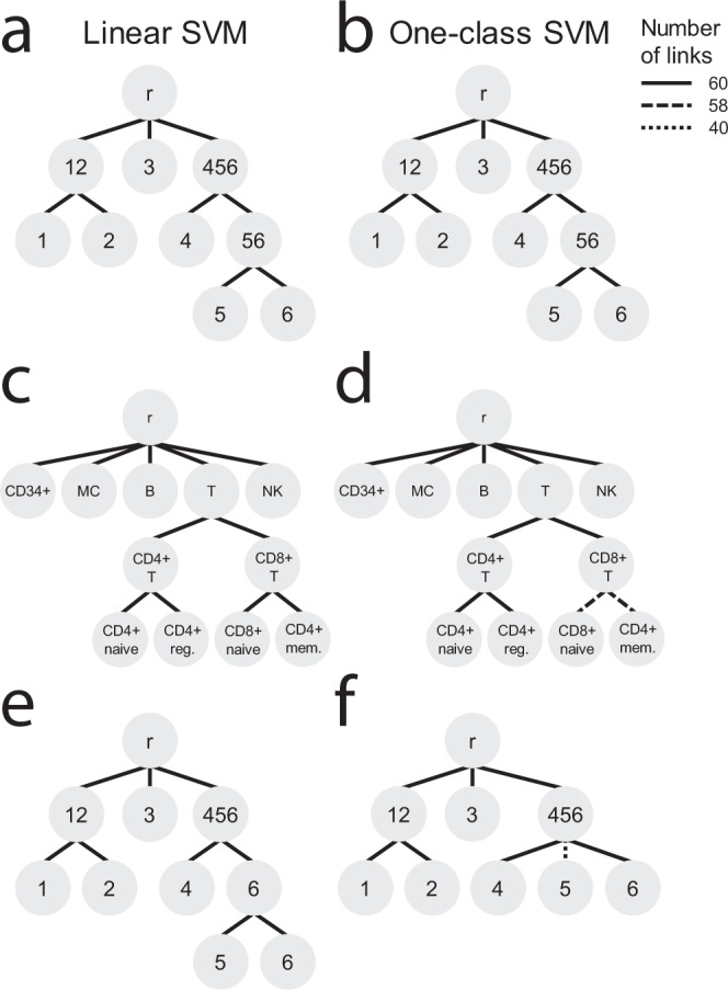
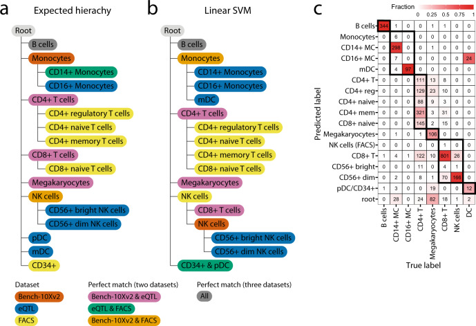
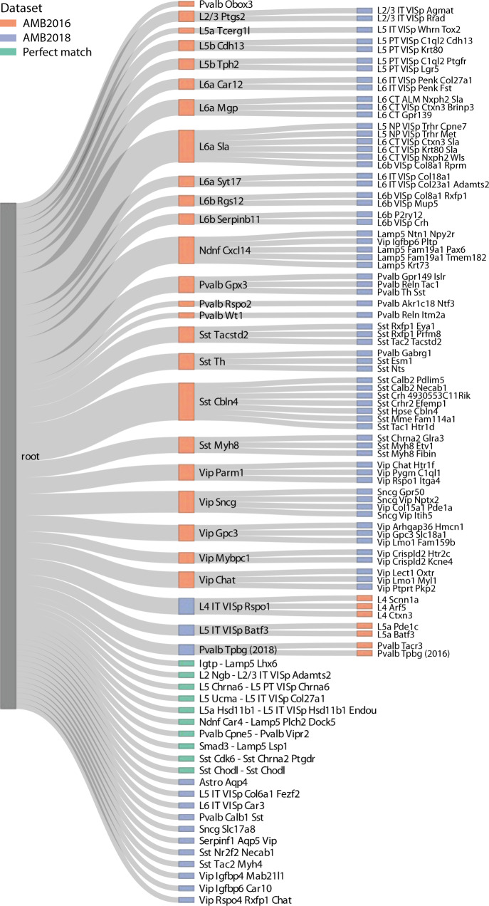
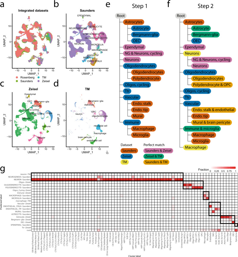
Supervised methods are increasingly used to identify cell populations in single-cell data. Yet, current methods are limited in their ability to learn from multiple datasets simultaneously, are hampered by the annotation of datasets at different resolutions, and do not preserve annotations when retrained on new datasets. The latter point is especially important as researchers cannot rely on downstream analysis performed using earlier versions of the dataset. Here, we present scHPL, a hierarchical progressive learning method which allows continuous learning from single-cell data by leveraging the different resolutions of annotations across multiple datasets to learn and continuously update a classification tree. We evaluate the classification and tree learning performance using simulated as well as real datasets and show that scHPL can successfully learn known cellular hierarchies from multiple datasets while preserving the original annotations. scHPL is available at https://github.com/lcmmichielsen/scHPL .

Fig. 1. Schematic overview of scHPL.

a Overview of the training phase. In the first iteration, we start with two labeled datasets. The colored areas represent the different cell populations. For both datasets a flat classifier (FC1 and FC2) is constructed. Using this tree and the corresponding dataset, a classifier is trained for each node in the tree except for the root. We use the trained classification tree of one dataset to predict the labels of the other. The decision boundaries of the classifiers are indicated with the contour lines. We compare the predicted labels to the cluster labels to find matches between the labels of the two datasets. The tree belonging to the first dataset is updated according to these matches, which results in a hierarchical classifier (HC1). In dataset 2, for example, subpopulations of population “1” of dataset 1 are found. Therefore, these cell populations, “A” and “B”, are added as children to the “1” population. In iteration 2, a new labeled dataset is added. Again a flat classifier (FC3) is trained for this dataset and HC1 is trained on datasets 1 and 2, combined. After cross-prediction and matching the labels, we update the tree which is then trained on all datasets 1–3 (HC2). b The final classifier can be used to annotate a new unlabeled dataset. If this dataset contains unknown cell populations, these will be rejected.

Fig. 2. Schematic examples of different matching scenarios.

a Perfect match, b splitting, c merging, and d new population. The first two columns represent a schematic representation of two datasets. After cross-predictions, the matching matrix (X) is constructed using the confusion matrices (Methods). We update the tree based on X.

Fig. 3. Classification performance.

a–c Boxplots showing the HF1-score of the one-class and linear SVM during n-fold cross-validation on the a simulated (n = 10), b PBMC-FACS (n = 10), and c AMB (n = 5) dataset. In the boxplots, the middle (orange) line represents the median, the lower and upper hinge represents the first and third quartiles, and the lower and upper whiskers represent the values no further than 1.5 interquartile range away from the lower and upper hinge, respectively. d Barplot showing the percentage of true positives (TP), false negatives (FN), and false positives (FP) per classifier on the AMB dataset. For the TPs a distinction is made between correctly predicted leaf nodes and internal nodes. e Heatmap showing the percentage of unlabeled cells per classifier during the different rejection experiments. f Heatmap showing the F1-score per classifier per cell population on the AMB dataset. Gray indicates that a classifier never predicted a cell to be of that population.

Fig. 4. Tree learning evaluation.

Classification trees learned when using a a, c, e linear SVM or b, d, f one-class SVM during the a, b simulated, c, d PBMC-FACS, and e, f simulated rejection experiment. The line pattern of the links indicates how often that link was learned during the 60 training runs. d In 2/60 trees, the link between the CD8+ T cells and the CD8+ naive and CD4+ memory T cells is missing. In those trees, the CD8+ T cells and CD8+ naive T cells have a perfect match and the CD4+ memory T cells are missing from the tree. f In 20/60 trees, the link between “Group456” and “Group5” is missing. In those trees, these two populations are a perfect match.

Fig. 5. PBMC inter-dataset evaluation.

a Expected and b learned classification tree when using a linear SVM on the PBMC datasets. The color of a node represents the agreement between dataset(s) regarding that cell population. c Confusion matrix when using the learned classification tree to predict the labels of PBMC-Bench10Xv3. The dark boundaries indicate the hierarchy of the constructed classification tree.

Fig. 6. Constructed hierarchy for the AMB datasets.

Learned classification tree after applying scHPL with a linear SVM on the AMB2016 and AMB2018 datasets. A green node indicates that a population from the AMB2016 and AMB2018 datasets had a perfect match. Three populations from the AMB2018 dataset are missing from the tree: “Pvalb Sema3e Kank4”, “Sst Hpse Sema3c”, and “Sst Tac1 Tacr3”.

Fig. 7. Brain inter-dataset evaluation.

a–d UMAP embeddings of the datasets after alignment using Seurat v3. e Learned hierarchy when starting with the Saunders dataset and adding Zeisel with linear SVM. f Updated tree when the Tabula Muris dataset is added. g Confusion matrix when using the learned classification tree to predict the labels of Rosenberg. The dark boundaries indicate the hierarchy of the classification tree.