Two-dimensional Bayesian inversion of magnetotelluric data using trans-dimensional Gaussian processes

Abstract

Bayesian inversion of electromagnetic data produces crucial uncertainty information on inferred subsurface resistivity. Due to their high computational cost, however, Bayesian inverse methods have largely been restricted to computationally expedient 1-D resistivity models. In this study, we successfully demonstrate, for the first time, a fully 2-D, trans-dimensional Bayesian inversion of magnetotelluric (MT) data. We render this problem tractable from a computational standpoint by using a stochastic interpolation algorithm known as a Gaussian process (GP) to achieve a parsimonious parametrization of the model vis-a-vis the dense parameter grids used in numerical forward modelling codes. The GP links a trans-dimensional, parallel tempered Markov chain Monte Carlo sampler, which explores the parsimonious model space, to MARE2DEM, an adaptive finite element forward solver. MARE2DEM computes the model response using a dense parameter mesh with resistivity assigned via the GP model. We demonstrate the new trans-dimensional GP sampler by inverting both synthetic and field MT data for 2-D models of electrical resistivity, with the field data example converging within 10 d on 148 cores, a non-negligible but tractable computational cost. For a field data inversion, our algorithm achieves a parameter reduction of over 32× compared to the fixed parameter grid used for the MARE2DEM regularized inversion. Resistivity probability distributions computed from the ensemble of models produced by the inversion yield credible intervals and interquartile plots that quantitatively show the non-linear 2-D uncertainty in model structure. This uncertainty could then be propagated to other physical properties that impact resistivity including bulk composition, porosity and pore-fluid content.

Keywords: Electrical properties; Inverse theory; Magnetotellurics; Non-linear electromagnetics; Probability distributions.

Figure 1.

Description of the high performance computing implementation and workflow of the trans-D MCMC algorithm. Loading the data and the dense finite element parameter mesh is handled in MARE2DEM. At iteration n, Birth-death MCMC (step 1), the parsimonious to dense GP transformation (step 2), and the acceptance/rejection of the proposed next model (step 5) are performed on the parsimonious model, , which provides the GP mean through eq. (9), on the manager CPU of the compute node, in Julia. Forward modelling in MARE2DEM (step 3) and misfit calculation (step 4) are performed on the dense model () on the worker CPUs, in Fortran. Communication between Julia and Fortran is handled through a direct Julia-to-Fortran interface subroutine. The numbers 1–5 represent the chronological order of operations at each iteration, as described in the text.

Figure 2.

Resistivity model from which synthetic data were generated. The model consists of shallow, extrusive volcanics overlying a resistive lithosphere and conductive asthenosphere. A conductive anomaly at the base of the lithosphere represents a partial melt prism. Synthetic data were generated at 11 MT sites (white triangles) over a period range of 10–10 000 s. The model grid consists of 818 independent resistivity cells.

Figure 3.

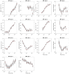
Synthetic TE (red circles) and TM (blue circles) mode apparent resistivity and phase for 11 MT sites (see white triangles in Fig. 2). In addition, the forward responses for 50 randomly selected models from the posterior ensemble are plotted in grey (TE mode) and blue (TM mode). The distribution of the RMS fit to the data across the ensemble had a mode of 1.25.

Figure 4.

Smooth resistivity model obtained from regularized inversion of the synthetic MT data using MARE2DEM. The smooth model indicates the scale of features resolvable by the data and can assist in selecting a resistivity mesh (outlined in black) sufficiently dense to capture the model complexity, as well as appropriate choices for the GP correlation length scales. Smooth versions of the main features of the melt prism model are present in the regularized estimate, including the extrusive volcanics, lithosphere, melt prism, and asthenosphere. The LAB is not sharply resolved.

Figure 5.

Synthetic inversion results. (a) The mean of the model ensemble captures the conductive melt prism (black box). The LAB (thin black line) is less well resolved. The resistivity mesh (outlined in black) and the interpolation node locations (black dots) for a model selected at random from the model ensemble are shown. (b) The marginal posterior distribution between 60 and 80 km depth [the region between the horizontal dashed lines in (a)] indicates that the uncertainty in the distribution beneath the conductive melt prism is greater than on either side of it. The true model values are indicated by white squares. (c) Marginal distribution through the melt prism [the region between the vertical dashed lines in (a)] shows a tightening of the uncertainty where the model is conductive, relative to where it is resistive. The red lines represent the 5th and 95th percentiles, and indicate the 90 per cent credible interval.

Figure 6.

Gemini MT data inversion results. (a) Deterministic inversion of the Gemini data, obtained using MARE2DEM. (b) Mean of the TDGP model ensemble. The dense resistivity mesh is outlined in black, while the interpolation node locations for a model randomly chosen from the ensemble are shown in (b) as black circles. The MT sites are represented by white triangles, in order from station 1 on the left to station 7 on the right. The uncertainty on the base of the salt (blue object in the center) is one of the key questions left unresolved by this inversion. The similarities between (a) and (b) are striking given the highly varied nature of the models in the ensemble (Fig. 10). Note the use of a linear colour scale given the small range of inverted resistivity.

Figure 7.

Gemini TE mode apparent resistivity and phase for 7 MT sites (see white triangles in Fig. 6). In addition, the forward responses for 50 randomly selected models from the ensemble are plotted in grey. The distribution of the RMS fit to the data across the ensemble was 1.1–1.5, with a peak at 1.28.

Figure 8.

Transformation from linear depth (km) to sampled depth, , given in eq. (15). The choice of b and c determines the fraction of a given interval in the transformed domain that maps to shallow depths in the untransformed domain. The dashed lines indicate for each combination of b and c the point (, ), the linear depth that corresponds to the midpoint of .

Figure 9.

Convergence properties of the trans-D GP inversion of the Gemini data set. Convergence properties (RMS misfit, number of interpolation nodes, and acceptance rates for the birth, death, resistivity update and position update moves) as a function of MCMC iteration number for the three Markov chains at temperature T= 1 are plotted in green, orange and blue. Histograms of these properties across all three chains are shown beneath. Models in the ensemble fit the data in the range RMS 1.1–1.5. The bulk of the models contained 125–475 interpolation nodes, compared with 8424 finite elements used by MARE2DEM.

Figure 10.

Several resistivity models chosen at random from the model ensemble, evaluated at the gridpoints. Despite the wide degree of variability, the mean of the ensemble coherently images the salt body. The degree of variability provides crucial knowledge of uncertainty in the subsurface resistivity. For example, note how in the vicinity of the magenta square there is always a resistor; similarly, in the vicinity of the white square there is always a conductor, whereas in some other locations the model exhibits more variability among the samples shown here (e.g. the tan circle).

Figure 11.

Marginal distributions for subsurface resistivity taken at various depth slices through the model: (a) 1.2–1.4 km; (b) 2.5–3.5 km; (c) 4.5–6.0 km and (d) 8.0–10.0 km. Warmer colours indicate higher probability density while the red lines denote the 90 per cent credible interval. The white squares represent gradient-based resistivity estimates at the gridoints within the depth slice. In general, model regions consistent with the salt body (brown shaded regions) exhibit an increase in the 5th percentile to above 1 Ωm, while regions consistent with sediments (pink shaded regions) have a 5th percentile that is significantly lower.

Figure 12.

Marginal distributions for subsurface resistivity taken at various vertical slices through the model: (a) –5 to –3 km; (b) –0.5 to 0.5 km; (c) 4.5 to 5.5 km and (d) 7.5 to 8.5 km. Warmer colours indicate higher probability density while the red lines denote the 90 per cent credible interval. The white squares represent gradient-based resistivity estimates at the gridpoints within the depth slice. In general, model regions consistent with the salt body (brown shaded regions) exhibit an increase in the 5th percentile to above 1 Ωm, while regions consistent with sediments (pink shaded regions) have a 5th percentile that is significantly lower.

Figure 13.

Interquartile range of the model ensemble obtained by TDGP inversion of the Gemini data set. Higher uncertainty generally occurs in the more resistive parts of the model (upper and lower salt bodies). Relative high uncertainty also occurs in the very shallow parts of the model where structure is shallower than the skin depths at the shortest periods for each station’s data (shown as white triangles labelled 1–7). The transition between sediments to salt appears clearly demarcated.

References

1. Agostinetti N.P., Bodin T., 2018. Flexible coupling in joint inversions: a Bayesian structure decoupling algorithm, J. geophys. Res., 123(10), 8798–8826. 10.1029/2018JB016079 - DOI - PMC - PubMed
1. Agostinetti N.P., Malinverno A., 2010. Receiver function inversion by trans-dimensional Monte Carlo sampling, J. geophys. Int., 181(2), 858–872.
1. Agostinetti N.P., Giacomuzzi G., Malinverno A., 2015. Local three-dimensional earthquake tomography by trans-dimensional Monte Carlo sampling, J. geophys. Int., 201(3), 1598–1617. 10.1093/gji/ggv084 - DOI
1. Bezanson J., Edelman A., Karpinski S., Shah V.B., 2017. Julia: a fresh approach to numerical computing, SIAM Rev., 59(1), 65–98. 10.1137/141000671 - DOI
1. Blatter D., 2020, Constraining fluid properties in the mantle and crust using Bayesian inversion of electromagnetic data, PhD thesis, Columbia University, New York City.