In vivo Morphometry of Inner Plexiform Layer (IPL) Stratification in the Human Retina With Visible Light Optical Coherence Tomography

Abstract

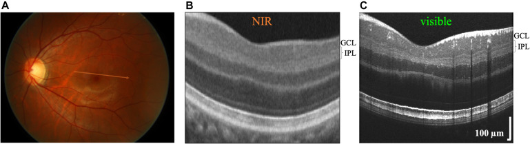
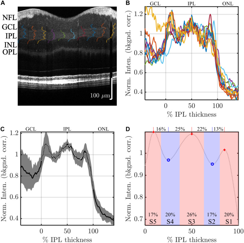
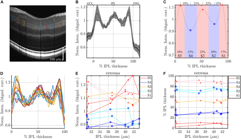
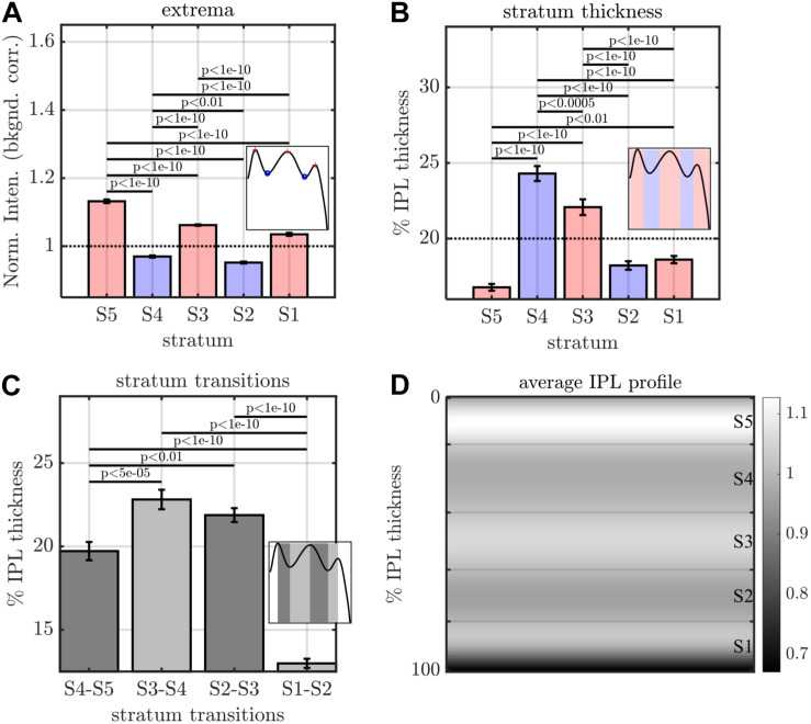
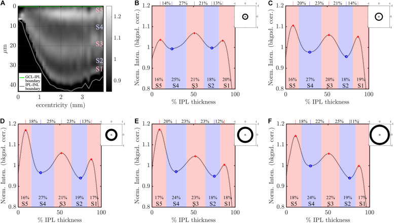
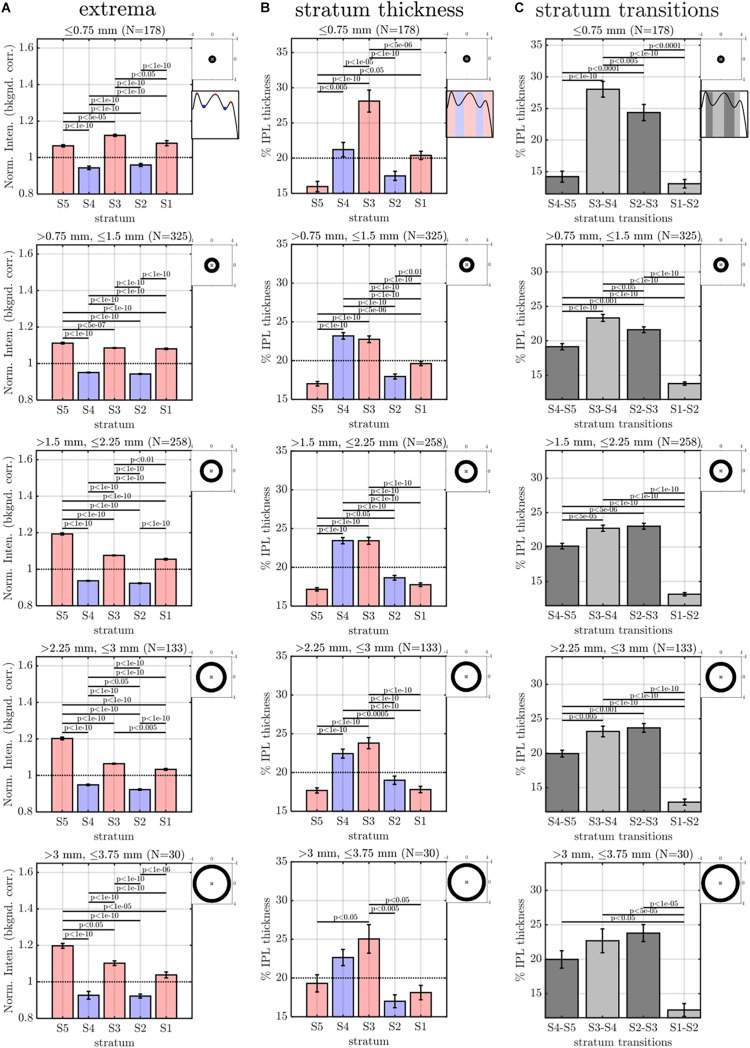
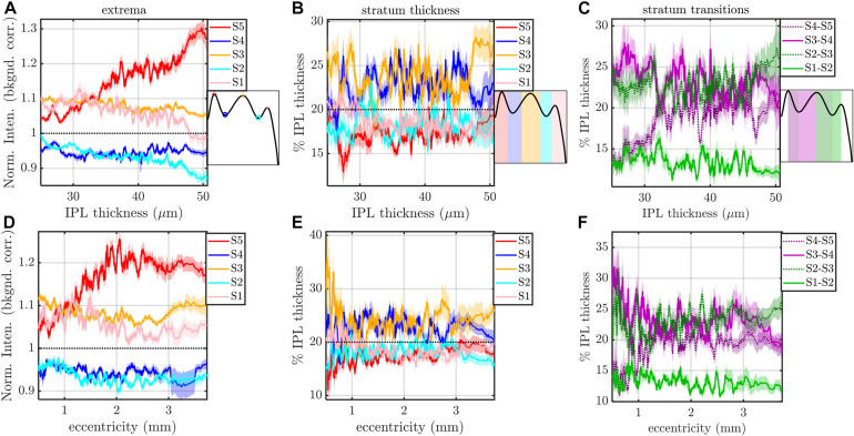
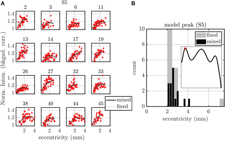
From the bipolar cells to higher brain visual centers, signals in the vertebrate visual system are transmitted along parallel on and off pathways. These two pathways are spatially segregated along the depth axis of the retina. Yet, to our knowledge, there is no way to directly assess this anatomical stratification in vivo. Here, employing ultrahigh resolution visible light Optical Coherence Tomography (OCT) imaging in humans, we report a stereotyped reflectivity pattern of the inner plexiform layer (IPL) that parallels IPL stratification. We characterize the topography of this reflectivity pattern non-invasively in a cohort of normal, young adult human subjects. This proposed correlate of IPL stratification is accessible through non-invasive ocular imaging in living humans. Topographic variations should be carefully considered when designing studies in development or diseases of the visual system.

Keywords: bipolar cells; ganglion cells; inner plexiform layer; outer plexiform layer; retina; retinal lamination; synapses; visible light optical coherence tomography.

FIGURE 1

Commercial near-infrared (NIR) and visible Optical Coherence Tomography (OCT) of a 26 years old Asian male with brown-colored iris. (A) OCT generates cross-sectional images by scanning broad bandwidth light on the fundus of the retina. Commercial NIR OCT (B) and visible light OCT (C) images of similar retinal eccentricities, intersecting the foveal pit superior to the foveola. Compared to commercial NIR OCT, visible light OCT achieves fivefold finer axial resolution, which improves visualization of substrata within the inner plexiform layer (IPL). In the visible light OCT image, IPL stratification is evident everywhere except near the central foveal pit. The NIR OCT image (B) was cropped from a Zeiss Cirrus High Definition 5 Line Raster scan (approximate location shown on fundus image in A).

FIGURE 2

Image analysis: example analysis of IPL strata (S1-S5) in a high quality visible light OCT image. IPL intensity profiles (background corrected, averaged transversally over 1.5°, and normalized so the average IPL intensity is 1. are displayed across the image (A) and also plotted versus % IPL thickness (B). (C) Average IPL profile, excluding segments with an IPL thickness below 24 microns, across locations (mean ± SD) shows a stereotyped pattern with 3 peaks and 2 valleys. A polynomial fit approximates the average profile (light gray dotted line), providing estimates of both peak and valley (extrema) locations (D). In this example, the reflectivity peak at the center of S3 is broad, separated by 25 and 22% IPL thickness from the nearest inner and outer valleys, respectively, as shown on top of the plot. This broad peak is flanked by relatively narrower peaks at the centers of S1 and S5, which are separated from the nearest inner and outer valleys by only 13 and 16% IPL thickness, respectively. In agreement with this observation, a wider S3 was also noted, where stratum divisions were defined by positions where intensity crossed the midpoint between adjacent extrema (red and blue shading), as shown at the bottom of the plot.

FIGURE 3

Segmental analysis: example analysis of IPL segments to evaluate topography. (A) IPL intensity profiles (background corrected, averaged transversally over 1.5° segments, and normalized) are displayed across the image. As in Figure 2, the average IPL profile (B), with polynomial fit and derived stratification parameters (C), are shown. (D) To evaluate topography, individual 1.5° segments are analyzed. Each segmental polynomial fit (dotted lines in D) provides extrema (E) and their locations (F), using the image-averaged profile (C) as a template (see main text). Red crosses are segmental maxima and blue circles are segmental minima. This segmental analysis reveals variations in stratification with either IPL thickness (abscissa in E,F) or eccentricity. Data from consecutive segments are connected with dotted lines.

FIGURE 4

Image analysis of IPL lamination parameters across 96 images (16 eyes × 6 high quality radial images), derived from the averaging and fitting procedure shown in Figure 2. (A) A stereotyped reflectivity pattern is consistently observed. Stratum thickness (B) and inter-stratum transitions (C) suggest a broadening around S3–S4. (D) Average image profile (shown as intensity image) clearly depicts the major features (i.e. high intensity or prominent S5, broad S3 and S4, narrow S1 and S5. Horizontal lines denote stratum boundaries.

FIGURE 5

Eccentricity-wise averaging of segmental IPL profiles. (A) Subject-averaged IPL lamination image, obtained by partitioning IPL segments into 25 eccentricity bins, averaging IPL profiles and thicknesses within each bin, then for each eccentricity bin, rescaling the abscissa of the average segmental profile to the average IPL thickness. IPL profiles, averaged across wider eccentricity bins (B: 0.75–1.13 mm, C: 1.13–1.5 mm, D: 1.5–2.25 mm, E: 2.25–3 mm, F: 3–3.75 mm). Both the image (A) and the plotted profiles (B–F) suggest an increase in the prominence of S5 starting near the foveal edge (0.75 mm). Note that while averaging across subjects and within eccentricity bins yields smooth profiles, individual profiles may not align; therefore, stratum contrast is reduced in this figure relative to Figures 6A, 7A. Topographic images in (B–F) show annuli for eccentricity binning relative to the foveal center (“x”).

FIGURE 6

Eccentricity-wise summary of segmental IPL parameters, derived from the averaging and fitting procedure shown in Figure 3: extrema (A), thicknesses (B), and transitions between strata (C). Note that since segmental profiles are not averaged before determining extrema, stratum contrast is increased relative to Figure 5, though the trends remain consistent. Topographic images show annuli for eccentricity binning relative to the foveal center (“x”).

FIGURE 7

Rolling average (mean ± std. err., window size of 21) of IPL stratification parameters (extrema, thicknesses, and transitions) versus IPL thickness (A–C) and eccentricity (D–F). The most salient feature is an increase in the intensity of S5 with IPL thickness (A) and an increase and pleateau in the intensity of S5 with eccentricity (D). S3 and S4 are consistently thicker, regardless of IPL thickness (B) and eccentricity (E). In agreement with these findings, S2–S3 and S3–S4 transitions are broader than other inter-stratum transitions (C,F). An increase in the width of the S4–S5 transition (C,F) accompanies the increased extrafoveal prominence of S5 (A,D).

FIGURE 8

Summary of fixed (fixed intercept, slope, and quadratic term for each subject) and mixed (fixed intercept, slope, and quadratic term as well as random intercept, slope, and quadratic term for each subject) effects models, applied to S5 peak versus eccentricity. (A) Model fits are shown for each of the 16 subjects, with subject index in subplot titles. (B) Both fixed and mixed effects models predict a maximum of the parabolic S5 peak profile around 2.4 mm eccentricity. Models for all other stratification parameters are summarized in Table 1 (eccentricity as a predictor) and Table 2 (IPL thickness as a predictor).

FIGURE 9

Summary of fixed (fixed intercept and slope for each subject) and mixed (fixed intercept and slope, with independent random intercept and slope for each subject) effects models, applied to S4-S5 transition width versus IPL thickness. (A) Model fits are shown for each of the 16 subjects, with subject index in subplot titles. (B) Histogram of subject slopes from the fixed effects model shows a statistically significant positive slope. Similar analysis for other stratification parameters are summarized in Table 1 (eccentricity as a predictor) and Table 2 (IPL thickness as a predictor).

FIGURE 10

Visualization of outer plexiform layer (OPL) lamination (A) and inner plexiform layer (IPL) lamination (B) in the same high quality visible light OCT image. (C) Zooms show a pentalaminar IPL reflectivity pattern (green outline) and a trilaminar OPL reflectivity pattern (purple outline). (D) Anatomical diagram (reproduced with permission Wang et al., 2003) of retinal circuitry depicts ON-OFF IPL stratification and rod-cone OPL stratification, where the rod spherules are outer to the cone pedicles. Note that the diagram is drawn with bottom-up processing for consistency with the OCT image display (GC, ganglion cell; A, amacrine cell; M, Müller cell; H, horizontal cell; CB, cone bipolar cell; RB, rod bipolar cell; C, cone; R, rod).

References

1. Balasubramanian R., Gan L. (2014). Development of Retinal Amacrine Cells and Their Dendritic Stratification. Curr. Ophthalmol. Rep. 2 100–106. 10.1007/s40135-014-0048-2 - DOI - PMC - PubMed
1. Boycott B. B., Wässle H. (1991). Morphological Classification of Bipolar Cells of the Primate Retina. Eur. J. Neurosci. 3 1069–1088. 10.1111/j.1460-9568.1991.tb00043.x - DOI - PubMed
1. Cajal S. R. Y. (1893). La rétine des vertébrés. Cellule 9 119–257.
1. Campbell J. P., Zhang M., Hwang S. (2017). Detailed Vascular Anatomy of the Human Retina by Projection-Resolved Optical Coherence Tomography Angiography. Sci. Rep. 7:42201. 10.1038/srep42201 - DOI - PMC - PubMed
1. Curcio C. A., Allen K. A. (1990). Topography of ganglion cells in human retina. J. Comp. Neurol. 300 5–25. 10.1002/cne.903000103 - DOI - PubMed