Nonlinear control of networked dynamical systems

Abstract

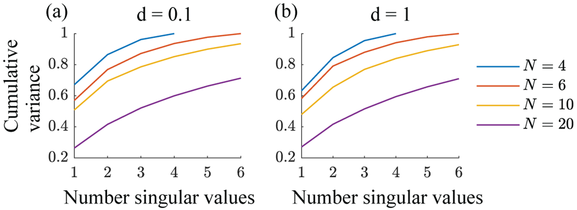
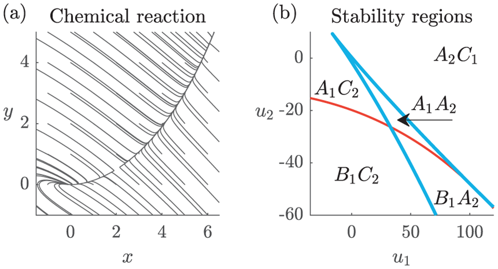
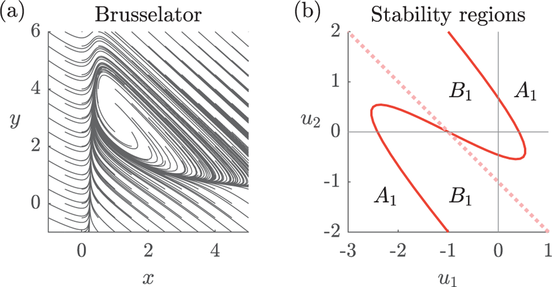
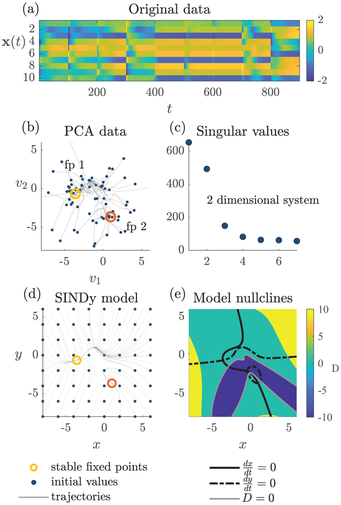
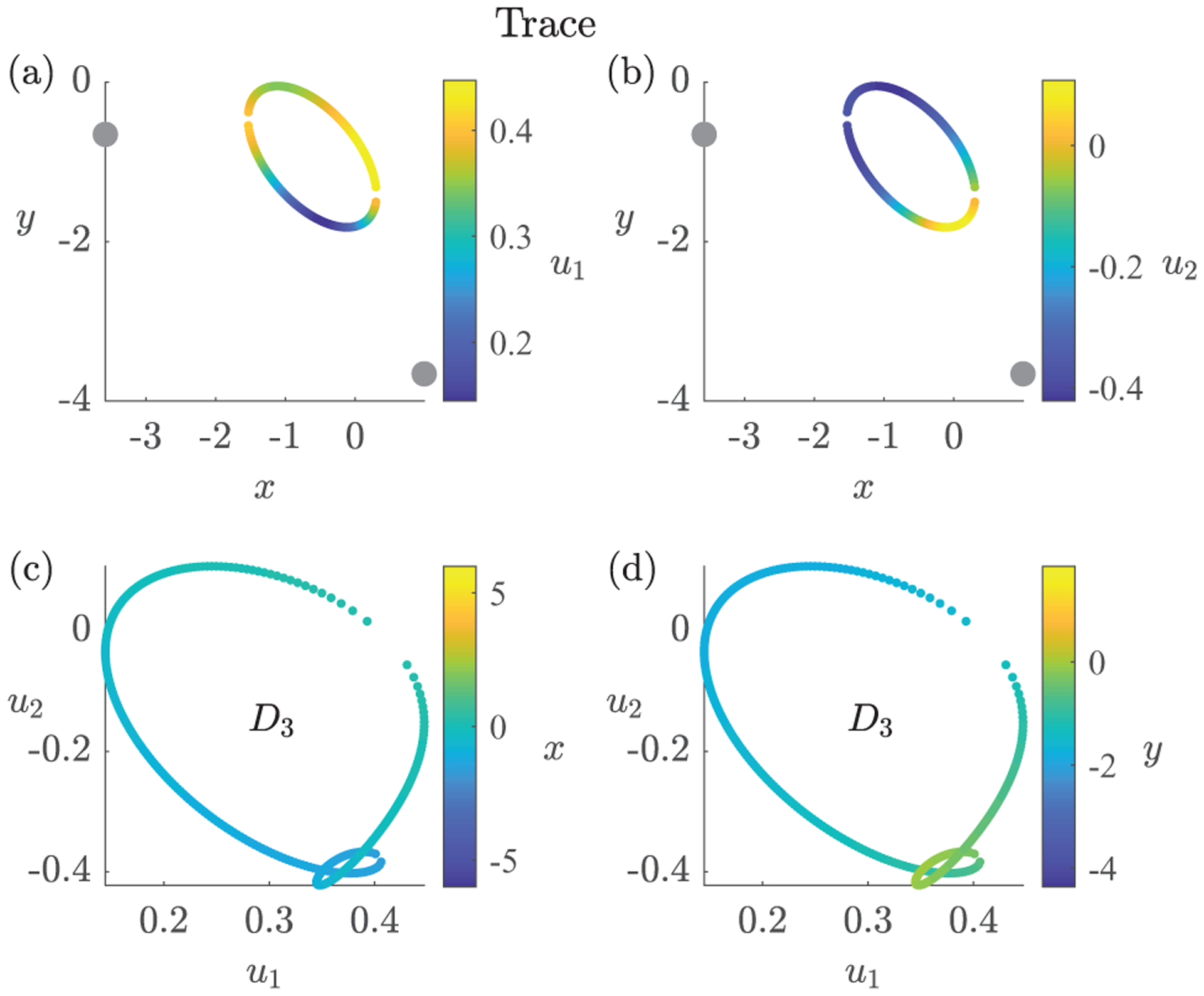
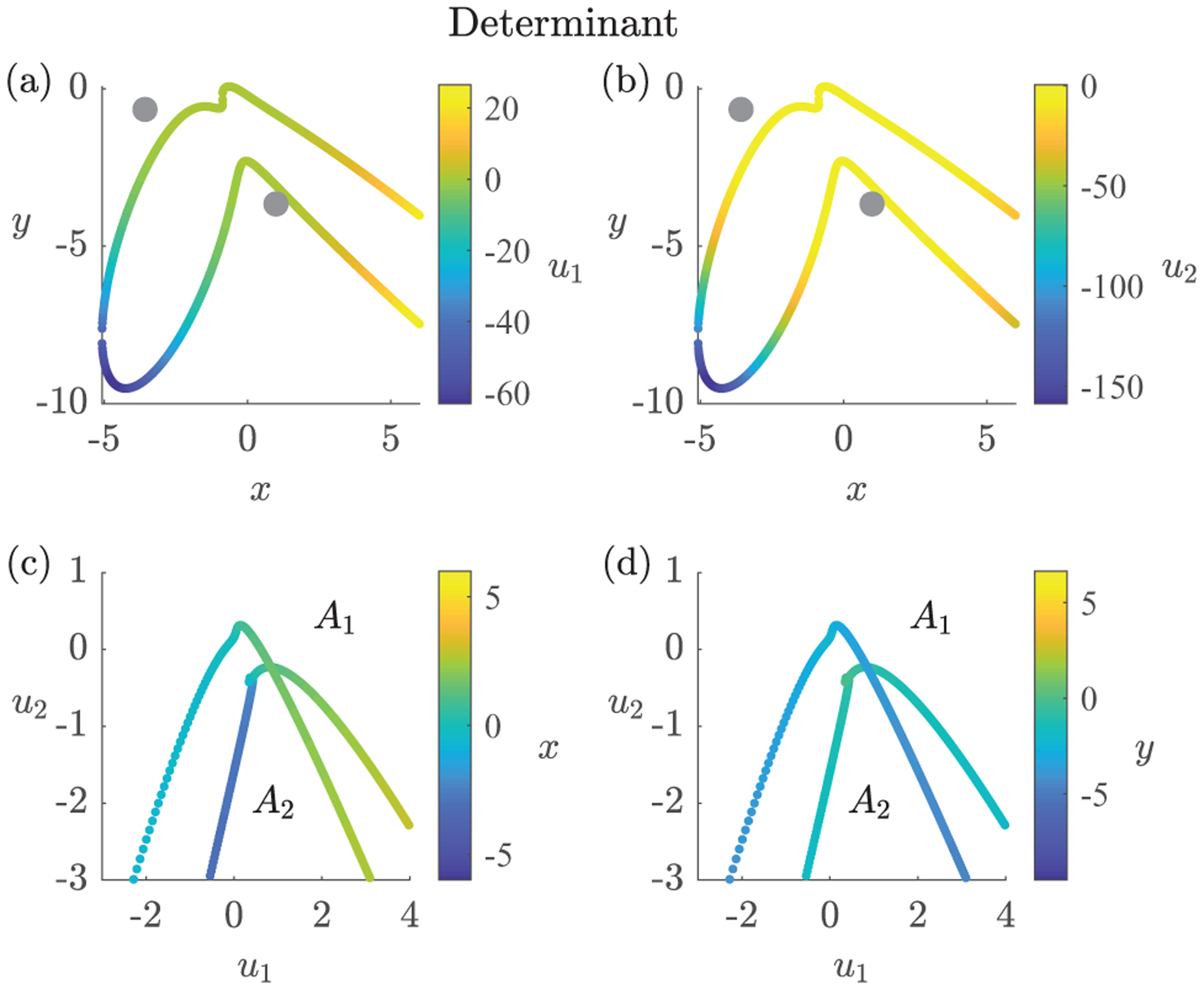
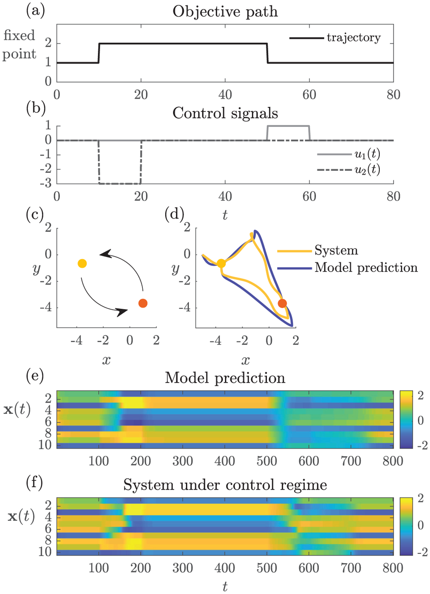
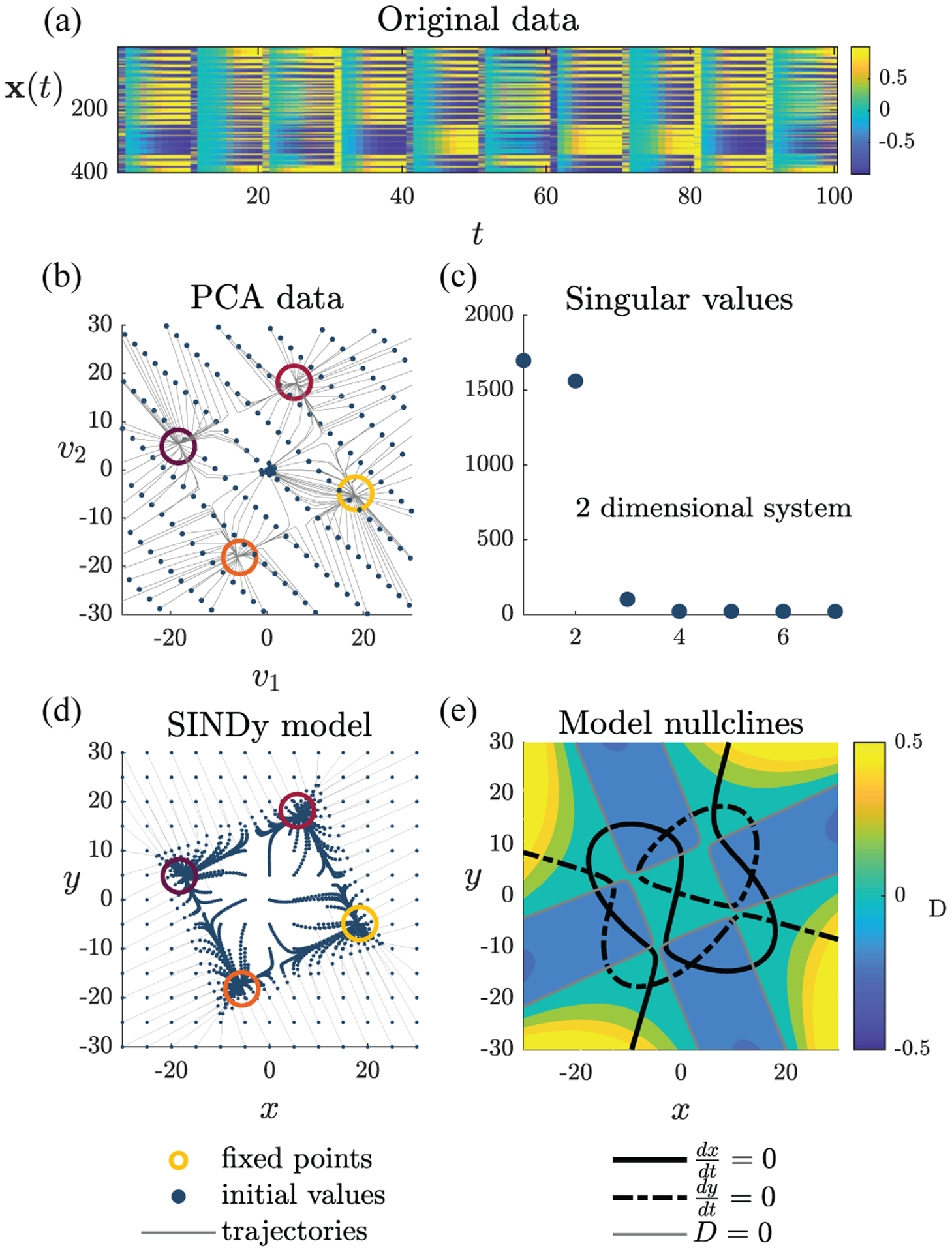
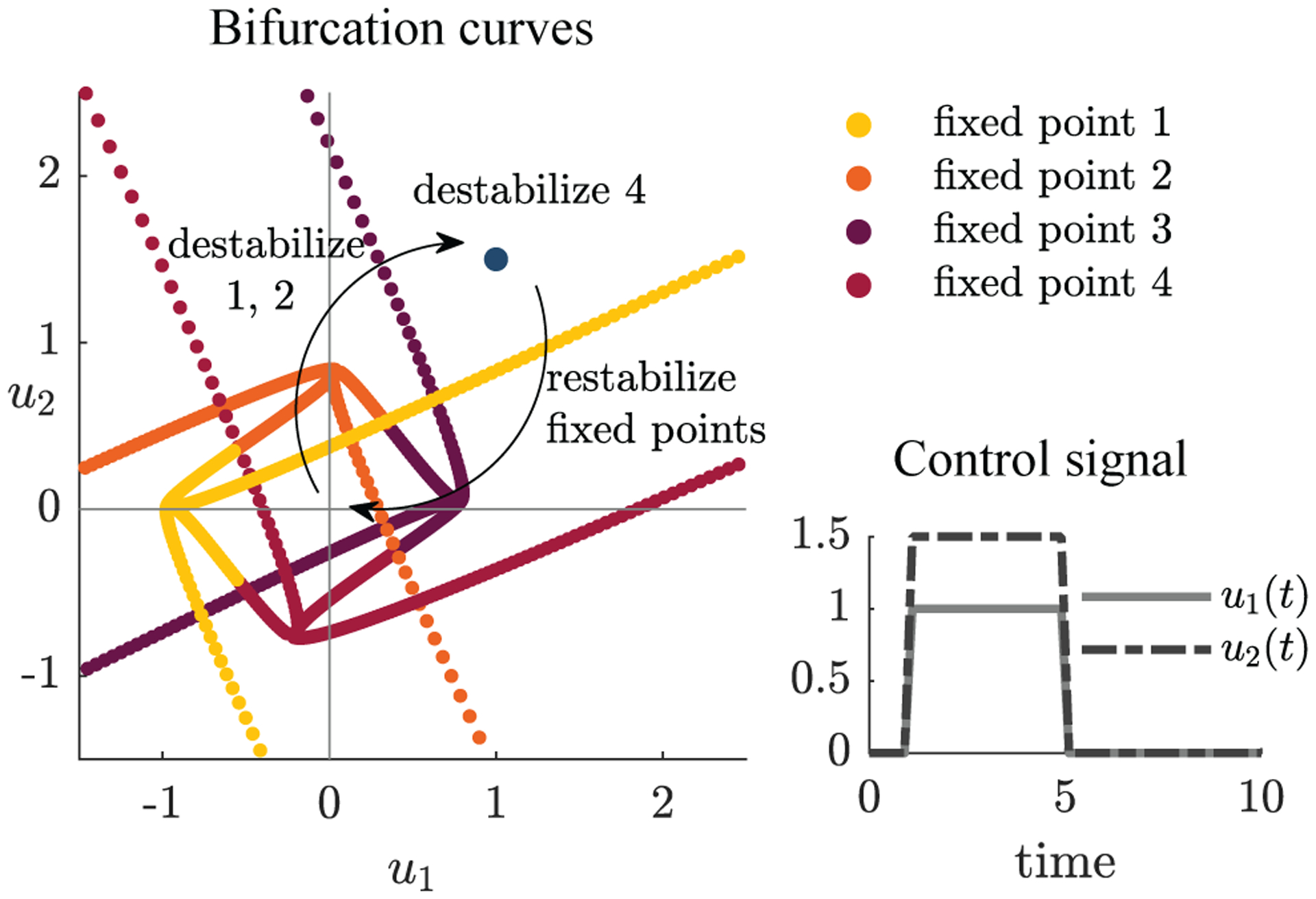
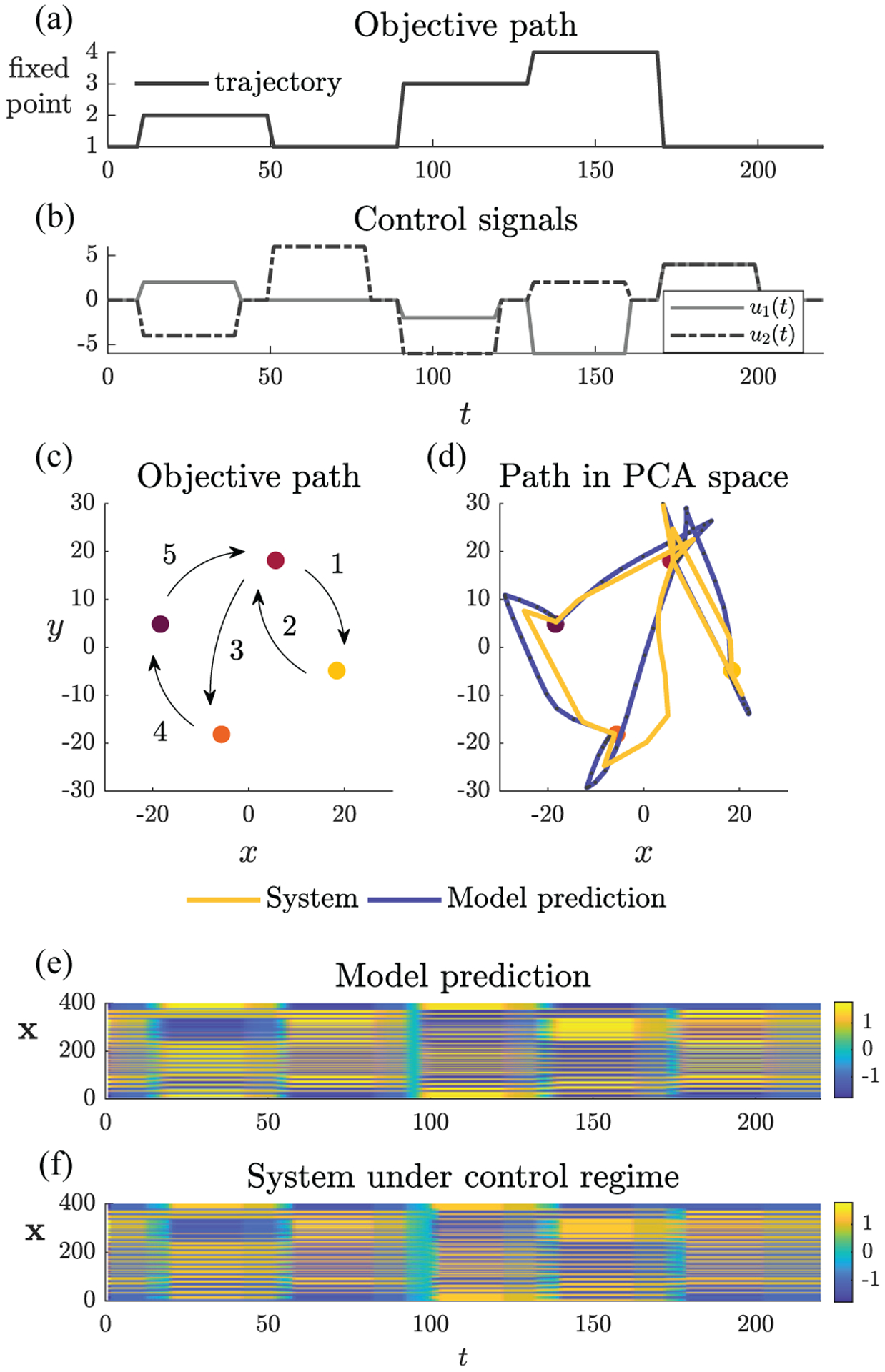
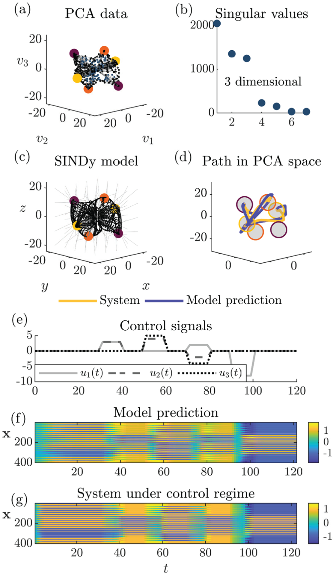
We develop a principled mathematical framework for controlling nonlinear, networked dynamical systems. Our method integrates dimensionality reduction, bifurcation theory, and emerging model discovery tools to find low-dimensional subspaces where feed-forward control can be used to manipulate a system to a desired outcome. The method leverages the fact that many high-dimensional networked systems have many fixed points, allowing for the computation of control signals that will move the system between any pair of fixed points. The sparse identification of nonlinear dynamics (SINDy) algorithm is used to fit a nonlinear dynamical system to the evolution on the dominant, low-rank subspace. This then allows us to use bifurcation theory to find collections of constant control signals that will produce the desired objective path for a prescribed outcome. Specifically, we can destabilize a given fixed point while making the target fixed point an attractor. The discovered control signals can be easily projected back to the original high-dimensional state and control space. We illustrate our nonlinear control procedure on established bistable, low-dimensional biological systems, showing how control signals are found that generate switches between the fixed points. We then demonstrate our control procedure for high-dimensional systems on random high-dimensional networks and Hopfield memory networks.

Keywords: Nonlinear control systems; bifurcation; limit-cycles; open-loop systems; pulse-based switching.

Fig. 1.

Average cumulative variance captured by initial singular values in random dynamical systems of increasing size N = 4, 6, 10, 20 [Appendix A]. (a) Dynamical systems consisting of a low percentage of possible term combinations, d = 0.1 (b) All possible term combinations included in the dynamical system, d = 1.0. Variance averaged over 100 trials

Fig. 2.

Regions of stability and instability for fixed points in a dynamical system. (a) Fixed points are sinks, sources, or saddles, depending on where they lie in the trace-determinant plane. (b) These regions map to stability regions in the control space. Movement across bifurcation curves in the control space correspond to moving between stability regions in the trace-determinant plane by crossing D = 0, T = 0, $\widehat{D}=0$, or $\widehat{T}=0$.

Fig. 3.

Chemical reaction with bistability. (a) In the absence of control signals there are two stable fixed points. (b) Regions of stability and instability for the fixed points in the uncontrolled system. The system has regions with two stable fixed points, one stable fixed point, a stable fixed point and a stable limit cycle, and only a stable limit cycle. Note the stable limit cycle appears surrounding the unstable source.

Fig. 4.

Brusselator (a) Brusselator with u₁, u₂ = 0. (b) Stability regions in the control space. The system transitions between having a single stable fixed point and an unstable source encapsulated by a stable limit cycle.

Fig. 5.

Low-dimensional model of a high dimensional random dynamical system. (a) High dimensional system n = 10 visualized as a timeseries and (b) shown in PCA space. (c) The first two PCA modes capture a reasonable amount of the data and the SINDy model (d) finds the two stable fixed points. (e) Nullclines and determinant of the SINDy model.

Fig. 6.

Fixed point locations and control signal values along the curve C^h(t) for the low-dimensional model found in Figure 5. (a-b) Fixed point locations in the xy-plane for C^h(t) colored by the u₁, u₂ control signal values along C^h(t). (c-d) Control signal locations in the u₁, u₂ plane for C^h(t) colored by (x, y) fixed point location values. The fixed point in this model that transitions across the curve T = 0 is the saddle fixed point that sits between the stable fixed points in the uncontrolled model. This saddle fixed point originally is located in region C₃ but transitions to region D₃ across the curve C^h(t).

Fig. 7.

Fixed point locations and control signal values along the curve C^s(t) for the low-dimensional model found in Figure 5. (a-b) Fixed point locations in the xy-plane for C^s(t) colored by the u₁, u₂ control signal values along C^s(t). (c-d) Control signal locations in the u₁, u₂ plane for C^s(t) colored by (x, y) fixed point location values. The fixed points in this model that transition across the curve D = 0 are the stable fixed points in the uncontrolled model. The right stable fixed point goes through a saddle-node bifurcation along the top curve, while the left stable fixed point goes through a saddle-node bifurcation along the bottom curve.

Fig. 8.

Control example for the random system in Figure 5. (a) Objective path for the system. (b) Control signals selected using the system’s stability region maps to move the system between fixed points. (c) Objective path in PCA space. (d) Predicted and actualized system paths in PCA space. (e-f) Predicted and actualized system activity in the original high-dimensional space.

Fig. 9.

Smooth Hopfield network size n = 400 with intrinsic 2-dimensional structure. (a) High-dimensional data measured from many initial conditions. (b) Data in PCA space. The network converges to one of 4 “memories”. (c) The first 2 modes capture the majority of the variance in the system. (d) SINDy is able to generate a low-dimensional model with similar dynamics that we can use to generate stability regions. (e) Nullclines and determinant of the SINDy model.

Fig. 10.

Saddle-node bifurcation curves C^s(t) colored by fixed point for the system in Figure 9. Moving across the saddle-node bifurcation curve of a stable fixed point either eliminates it from the system or reinstates it.

Fig. 11.

Control example for the hopfield system in Figure 9. (a) Objective path for the system. (b) Control signals selected using the systems’s stability region maps to move the system between fixed points. (c) Objective path in PCA space. (d) Predicted and actualized system paths in PCA space. (e-f) Predicted and actualized system activity in the original high-dimensional space.

Fig. 12.

Smooth Hopfield network size n = 400 with intrinsic 3-dimensional structure. (a) Hopfield data in PCA space. The network converges to one of 6 “memories”. (b) The first 3 modes capture the majority of the variance in the system. (c) SINDy is able to capture a low-dimensional model with similar dynamics that we can use to construct a control regime. (d) Predicted and actualized network activity in PCA space. (e) There are now 3 control signals in the control regime as we are using a 3-dimensional system. (f-g) Predicted and actualized network activity in the original space under the specified control regime.

Fig. 13.

Randomly generated high-dimension system n = 20 with a strange attractor. (a) SINDy model with 3 variables captures the stable fixed points and strange attractor in the system. (b) Predicted and actualized network activity in PCA space under control. (c) Predicted and actualized network activity in the high-dimensional space. Notice that although the SINDy model captured the location of the strange attractor, it does not adequately capture its frequency as the model predicts a much slower oscillation that the original system actually produces.

References

1. Jones LM, Fontanini A, Sadacca BF, Miller P, and Katz DB, “Natural stimuli evoke dynamic sequences of states in sensory cortical ensembles,” Proceedings of the National Academy of Sciences, vol. 104, no. 47, pp. 18772–18777, 2007, publisher: National Acad Sciences. - PMC - PubMed
1. Rabinovich M, Huerta R, and Laurent G, “Transient dynamics for neural processing,” Science, vol. 321, no. 5885, pp. 48–50, 2008, publisher: American Association for the Advancement of Science. - PubMed
1. Brunton SL and Kutz JN, Data-driven science and engineering: machine learning, dynamical systems, and control. Cambridge, United Kingdom; New York, NY: Cambridge University Press, 2019.
1. Kato S, Kaplan H, Schrödel T, Skora S, Lindsay T, Yemini E, Lockery S, and Zimmer M, “Global brain dynamics embed the motor command sequence of Caenorhabditis elegans,” Cell, vol. 163, no. 3, pp. 656–669, Oct. 2015. [Online]. Available: https://linkinghub.elsevier.com/retrieve/pii/S0092867415011964 - PubMed
1. Marvel SA, Kleinberg J, Kleinberg RD, and Strogatz SH, “Continuous-time model of structural balance,” PNAS, vol. 108, no. 5, pp. 1771–1776, Feb. 2011. [Online]. Available: http://www.pnas.org/content/108/5/1771 - PMC - PubMed
LinkOut - more resources