SPHERIOUSLY? The challenges of estimating sphere radius non-invasively in the human brain from diffusion MRI

Abstract

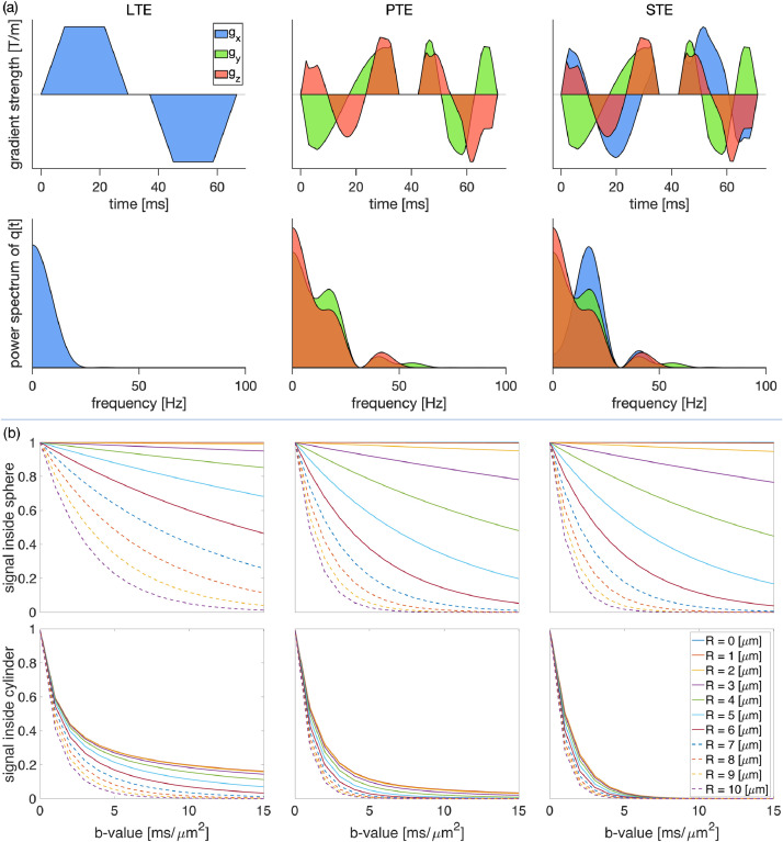
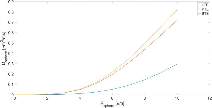
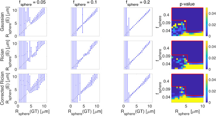
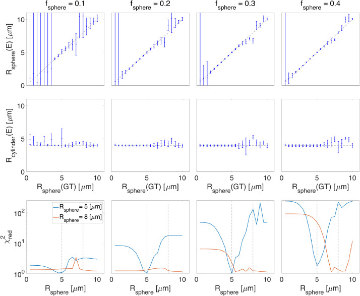
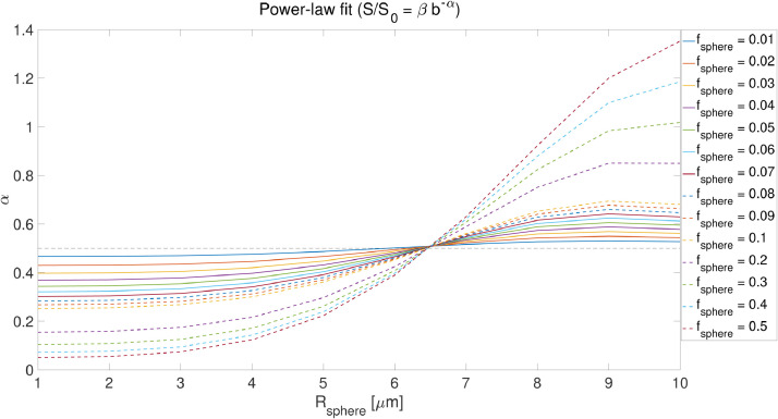
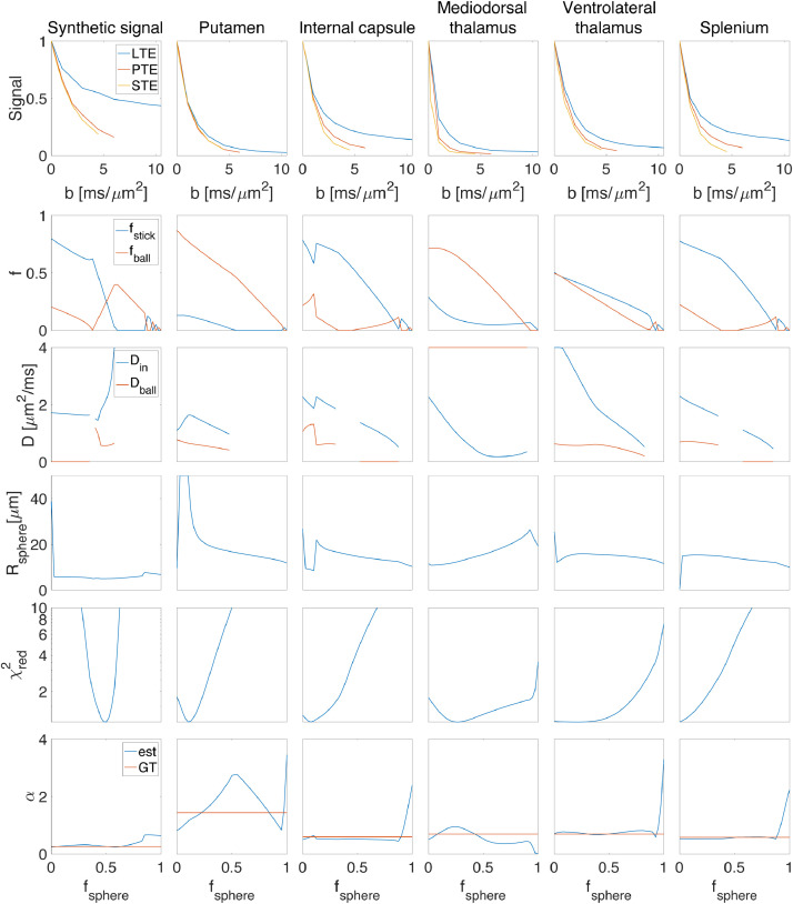
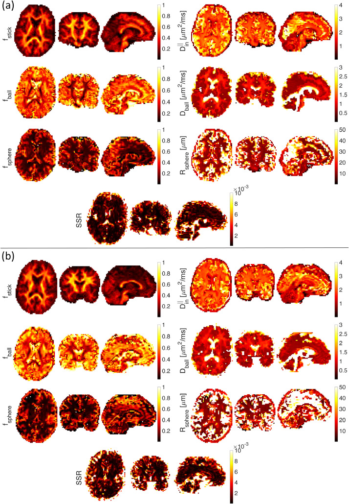
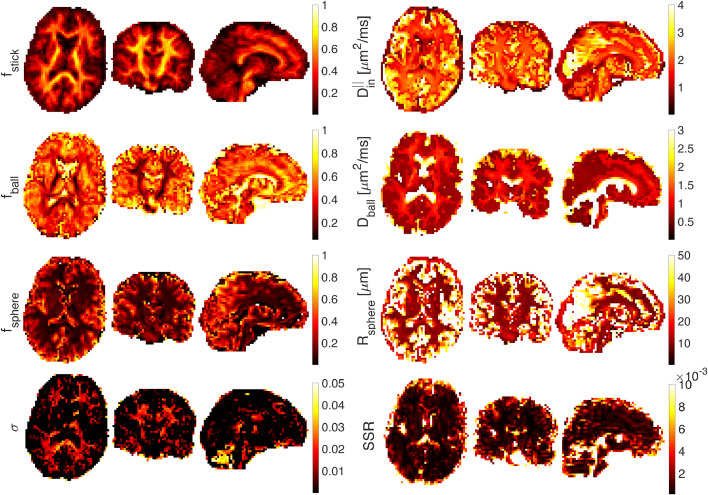
The Soma and Neurite Density Imaging (SANDI) three-compartment model was recently proposed to disentangle cylindrical and spherical geometries, attributed to neurite and soma compartments, respectively, in brain tissue. There are some recent advances in diffusion-weighted MRI signal encoding and analysis (including the use of multiple so-called 'b-tensor' encodings and analysing the signal in the frequency-domain) that have not yet been applied in the context of SANDI. In this work, using: (i) ultra-strong gradients; (ii) a combination of linear, planar, and spherical b-tensor encodings; and (iii) analysing the signal in the frequency domain, three main challenges to robust estimation of sphere size were identified: First, the Rician noise floor in magnitude-reconstructed data biases estimates of sphere properties in a non-uniform fashion. It may cause overestimation or underestimation of the spherical compartment size and density. This can be partly ameliorated by accounting for the noise floor in the estimation routine. Second, even when using the strongest diffusion-encoding gradient strengths available for human MRI, there is an empirical lower bound on the spherical signal fraction and radius that can be detected and estimated robustly. For the experimental setup used here, the lower bound on the sphere signal fraction was approximately 10%. We employed two different ways of establishing the lower bound for spherical radius estimates in white matter. The first, examining power-law relationships between the DW-signal and diffusion weighting in empirical data, yielded a lower bound of 7μm, while the second, pure Monte Carlo simulations, yielded a lower limit of 3μm and in this low radii domain, there is little differentiation in signal attenuation. Third, if there is sensitivity to the transverse intra-cellular diffusivity in cylindrical structures, e.g., axons and cellular projections, then trying to disentangle two diffusion-time-dependencies using one experimental parameter (i.e., change in frequency-content of the encoding waveform) makes spherical radii estimates particularly challenging. We conclude that due to the aforementioned challenges spherical radii estimates may be biased when the corresponding sphere signal fraction is low, which must be considered.

Keywords: Diffusion-weighted imaging; Direction-averaged diffusion signal; Spherical compartment; Three-compartment model; b-tensor encoding.

Fig. 1

Location of the five ROIs used for the quantitative analysis of this study overlaid on the FA image of one subject. The posterior limb of the internal capsule, splenium, putamen, ventrolateral thalamus, and mediodorsal thalamus are illustrated as red ROIs on the FA map.

Fig. 2

(a) The free gradient waveforms of the linear, planar, spherical tensor encoding and the corresponding frequency power spectra. (b) The signal decay inside the spherical and cylindrical compartments using different encoding schemes and different radii

Fig. 3

The changes in the apparent diffusivity ($D_{\text{sphere}}$) versus the radius of the sphere ($R_{\text{sphere}}$) for linear, planar and spherical tensor encoding (LTE, PTE, and STE)

Fig. 4

The results of fitting (stick + ball + sphere) the sphere radius for different sphere signal fractions (GT = Ground Truth and E = Estimated). The figure also shows the p-value of the F-test in the presence of Gaussian, Rician, and corrected Rician noise respectively. The red rectangles in the right side plots show the areas that the three-compartment model is significantly different from the two-compartment model (three-compartment model (stick + ball + sphere) is preferred over the two-compartment model (stick + ball)). The diagonal black line is the line of identity and the error bars show the confidence interval.

Fig. 5

Estimated sphere and cylinder radii versus the ground truth sphere radius values for cylinder + ball + sphere model ($SNR=200$). The third row shows the reduced chi-square, ${\chi }_{\text{red}}^2$, values for two scenarios where the sphere radius is 5 and 8 $\mu m$, blue and red curves respectively We take the simulated signal generated for $R_{\mathrm{sphere}}=5$ and instead of estimating all the parameters of the model which are $f_{\mathrm{cylinder}}$, $f_{\mathrm{ball}}$, $f_{\mathrm{sphere}}$, $D_{\mathrm{in}}^{\mid \mid }$, $D_{\mathrm{ball}}$, $R_{\mathrm{sphere}}$, and $R_{\mathrm{cylinder}}$, we fix $R_{\mathrm{sphere}}$ to $0.5,1,1.5,...,10\mu m$ and estimate the remaining parameters and plot the reduced chi-square as a function of $R_{\mathrm{sphere}}$ (blue curve). If there is not degeneracy, we expect to see a sharp minimum in the ${\chi }_{\text{red}}^2$ curve at $R_{\mathrm{sphere}}=5$ which is clear in the figure. We repeat the same strategy for $R_{\mathrm{sphere}}=8\mu m$ (the red curve) where the ${\chi }_{\text{red}}^2$ curve has several local minima or even flat which shows the presence of degeneracy when $R_{\mathrm{sphere}}$ is larger than $5\mu m$. This behavior can be explained by the swap of time dependent parameters ($R_{\mathrm{sphere}}$ and $R_{\mathrm{cylinder}}$) in the fitting which leads to unstable fitting of the model parameters. (GT = ground truth and E = estimated).

Fig. 6

The effect of sphere size and signal fraction on exponent $\alpha$ (similar to Fig. 2 in (Palombo et al., 2018a)). ($f_{\text{sphere}}=0.01:0.01:0.1,0.2:0.1:0.5$, $f_{\text{ball}}=f_{\text{stick}}=(1-f_{\text{sphere}})/2$, $D_{\text{in}}^{\mid \mid }=2\mu m^2/ms$, $D_{\text{ball}}=1\mu m^2/ms$, $R_{\text{sphere}}=1:1:10\mu m$, $\delta =29.65ms$, and $\Delta =37.05ms$).

Fig. 7

The results of fitting the stick + ball + sphere model to the diffusion-weighted signal by fixing the sphere signal fraction to different values. Five different ROIs of the brain are used here; putamen, internal capsule, mediodorsal thalamus, ventrolateral thalamus, and splenium. The mean value of the direction-averaged signal for each ROI is represented in the first row (in different columns). The second row shows the estimated signal fraction of stick ($f_{\text{stick}}$) and ball ($f_{\text{ball}}$) for different predefined sphere signal fractions (We used $f$ as y-label here to show the signal fraction of both ball and stick in one plot). The third row illustrates the parallel diffusivity of the stick ($D_{\text{in}}^{\mid \mid }$) and the diffusivity of the ball ($D_{\text{ball}}$) for different ROIs. The estimated radius of the sphere is illustrated in the fourth row. And finally, the last two rows show how well this model can explain the signal for different predefined sphere signal fractions ($f_{\text{sphere}}$) in terms of reduced chi-square and power-law. The first column in the figure shows the results of fitting a synthetic signal generated with the following parameters; $f_{\text{sphere}}=0.5$, $f_{\text{ball}}=f_{\text{stick}}=0.25$, $D_{\text{in}}^{\mid \mid }=2\mu m^2/ms$, $D_{\text{ball}}=0.6\mu m^2/ms$, $R_{\text{sphere}}=5\mu m$, and SNR = 100, Rician distributed signal. Note that we do not estimate diffusivity of the compartment when the signal fraction is estimated as zero, this is the reason for discontinuity in the plots of estimated diffusivities.

Fig. 8

Ball+stick+sphere model without estimation of noise parameter. Estimated stick ($f_{\text{stick}}$), ball ($f_{\text{ball}}$), and sphere ($f_{\text{sphere}}$) signal fractions, intra-axonal parallel diffusivity ($D_{\text{in}}^{\mid \mid }(\mu m^2/ms)$), extra-cellular diffusivity ($D_{\text{ball}}(\mu m^2/ms)$), and sphere radius ($R_{\text{sphere}}\left(\mu m\right)$) on axial, sagittal, and coronal views of the smoothed brain image ((a) first subject and (b) the second subject) (A 3D Gaussian kernel with standard deviation of 0.5 is used for smoothing).

Fig. 9

Ball+stick+sphere model with estimation of the noise parameter. Estimated stick ($f_{\text{stick}}$), ball ($f_{\text{ball}}$), and sphere ($f_{\text{sphere}}$) signal fractions, intra-axonal parallel diffusivity ($D_{\text{in}}^{\mid \mid }(\mu m^2/ms)$), extra-cellular diffusivity ($D_{\text{ball}}(\mu m^2/ms)$), sphere radius ($R_{\text{sphere}}\left(\mu m\right)$), and standard deviation of the noise ($\sigma$) on axial, sagittal, and coronal views of the smoothed brain image (A 3D Gaussian kernel with standard deviation of 0.5 is used for smoothing).

Fig. 10

Estimated FA, parameter $\beta$ and $\alpha$ of the power-law fit ($S/S_0=\beta b^{-\alpha }$) from axial, coronal, and sagittal views of the brain image.

References

1. Afzali M., Aja-Fernández S., Jones D.K. Direction-averaged diffusion-weighted MRI signal using different axisymmetric B-tensor encoding schemes. Magnetic Reson. Med. 2020 - PMC - PubMed
1. Afzali M., Knutsson H., Özarslan E., Jones D.K. Computing the orientational-average of diffusion-weighted mri signals: a comparison of different techniques. bioRxiv. 2020 - PMC - PubMed
1. Afzali M., Pieciak T., Newman S., Garifallidis E., Özarslan E., Cheng H., Jones D.K. The sensitivity of diffusion MRI to microstructural properties and experimental factors. J. Neurosci. Method. 2020:108951. - PMC - PubMed
1. Aja-Fernández S., Tristán-Vega A. Influence of noise correlation in multiple-coil statistical models with sum of squares reconstruction. Magnetic Reson. Med. 2012;67(2):580–585. - PubMed
1. Aja-Fernández S., Tristán-Vega A., Hoge W.S. Statistical noise analysis in grappa using a parametrized noncentral chi approximation model. Magnetic Resonan. Med. 2011;65(4):1195–1206. - PMC - PubMed
Publication types