Polynomial, piecewise-Linear, Step (PLS): A Simple, Scalable, and Efficient Framework for Modeling Neurons

Abstract

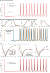
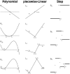
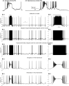
Biological neurons can be modeled with different levels of biophysical/biochemical details. The accuracy with which a model reflects the actual physiological processes and ultimately the information function of a neuron, can range from very detailed to a schematic phenomenological representation. This range exists due to the common problem: one needs to find an optimal trade-off between the level of details needed to capture the necessary information processing in a neuron and the computational load needed to compute 1 s of model time. An increase in modeled network size or model-time, for which the solution should be obtained, makes this trade-off pivotal in model development. Numerical simulations become incredibly challenging when an extensive network with a detailed representation of each neuron needs to be modeled over a long time interval to study slow evolving processes, e.g., development of the thalamocortical circuits. Here we suggest a simple, powerful and flexible approach in which we approximate the right-hand sides of differential equations by combinations of functions from three families: Polynomial, piecewise-Linear, Step (PLS). To obtain a single coherent framework, we provide four core principles in which PLS functions should be combined. We show the rationale behind each of the core principles. Two examples illustrate how to build a conductance-based or phenomenological model using the PLS-framework. We use the first example as a benchmark on three different computational platforms: CPU, GPU, and mobile system-on-chip devices. We show that the PLS-framework speeds up computations without increasing the memory footprint and maintains high model fidelity comparable to the fully-computed model or with lookup-table approximation. We are convinced that the full range of neuron models: from biophysical to phenomenological and even to abstract models, may benefit from using the PLS-framework.

Keywords: CPU; GPU; biophysical models; mobile devices; neurodynamics; neurons; phenomenological models.

Listing 2.1

Pseudo-code of lookup table implementation.

Figure 1

Constructing approximations of Wang and Buzsáki biophysical model. (A) Voltage traces for the original model (black line) overlapped with solution based upon lookup-table approximation (red line). (B) Top from left to right: Steady-state for fast sodium activation (m_∞(v)), inactivation (h_∞(v)), and delay-rectifier potassium activation (n_∞(v)) and time constants for sodium inactivation (τ_h(v)) and potassium activation [τ_n(v)] for the original model and two approximations: black lines—original model, blue lines—5^th order polynomial interpolation, orange lines—piecewise-Linear approximation. Bottom: Voltage traces for the same approximations. (C) Top left: voltage nullclines at different applied currents (I = I_app) for the original model reduced to 2 dimensions. Top center: Construction of only polynomial (green line) or Polynomial+piecewise-Linear approximation (PL 2D, red dashed line) from the original model after the reduction (black line). Top right: nullclines for the PL2D model (the same color-code and applied currents as in the left plot) Bottom: Voltage traces for original model (black line) and PL2D approximation (red line).

Figure 2

Comparison of original Wang and Buzsáki model with different approximations. (A) FI-curves, used for accuracy assessment. (B1) Performance Of 3D lookup table (red), 3D piecewise-Linear (L, yellow), 3D Polynomial (P, green), and 2D Polynomial+piecewise-Linear approximations (PL2D, brown) in comparison with the original 3D model (blue) computed on four different platforms: CPU—Intel Core i5-5257U, RPI1—Raspberry Pi 1, RPI4—Raspberry Pi 4, and GPU—NVidia GeForce RTX 2080 Ti. (B2) Assessment of memory size needed for model constants in the total number of single, double, or long double precision numbers. (B3) Standard squared error between FI-curve of the original model and four different approximations.

Figure 3

Examples of functions, which comprise the PLS-framework.

Figure 4

Phase-Plane Analysis and dynamics for phenomenological models of Integrating and Resonant neurons. Phase-portrait (A) and time constants (B) for the integrator model with parameters: v₀ = −65 mV, v₁ = −45 mV, v₂ = 55 mV, a₀ = 3.5 10⁻⁶, a₁ = −10⁻⁴(mV)⁻¹, v₃ = −35 mV, r₀ = 0.04 ms, r₁ = −0.004 ms/mV, v₄ = −40 mV, v₅ = −5 mV, v₆ = −55.45 mV, v₇ = 18.78 mV, s₀ = 5 ms, s₁ = 7.6 ms, s₂ = 1.8 ms, k = 2. Voltage nullclines are shown for zero current at resting (blue curve), for saddle-node bifurcation at the onset of pacing (I₀, yellow curve), and for saddle-node bifurcation at the onset of depolarization block (I₁, red curve). (C) Protocol (top) and voltage trace (bottom) of integrator dynamics. The model was held almost at the bifurcation point (I₀) for 500 ms, and then the applied current slightly increases at the point marked by triangle for 9 s. At the last second, a ramp of the input current traverses from 0.9I₁ to 1.1I₁ to show the depolarization block. (D) Phase-plane analysis for the resonator, with the same as for integrator parameters except for v₁—is not used in this model, and a₀ = 3.25 10⁻⁶, v₄ = −75 mV, v₅ = −5 mV, v₆ = −55.5 mV, v₇ = 18 mV. Voltage nullclines are shown for zero current at resting (blue curve), for Andronov-Hopf bifurcation (I₀, yellow curve), and for saddle-node bifurcation at the onset of depolarization block (I₁, red curve). (E) Dynamics of the resonator. The protocol is the same as for the integrator.

Listing 3.1

Implementation of PLS functions in C-language.

Listing 3.2

Implementation of PLS functions in Python.

Figure 5

Reproduction of immature, neuron-wide Plateau-Potential in five phenomenological models. (A1) Evoked and (A2) Spontaneous Plateau-Potentials recorded in vivo in rat visual cortex. Graphs reproduced from the data and by the scripts reported previously (Colonnese, 2014). (B) Five phenomenological models responses on input similar to dLGN neuron firing during the same period of the development. (B1) Izhikevich's model in regular firing mode, (B2) Exponential Leaky Integrate-and-Fire model with linear adaptation, (B3) Exponential Leaky Integrate-and-Fire model with non-linear adaptation, (B4) Type 1 neuron implemented in PLS-network (parameters are the same as in Figures 4A–C), (B5) Type 2 neuron implemented in PLS-network (parameters are the same as in Figures 4B,D,F). For each model, subplot BX.2 is the zoomed burst on subplot BX.1. Synaptic conductance was adjusted to obtain a realistic 0.7–1 Hz firing rate outside the burst. For (B3), synaptic conductance was set higher than the adjusted level in an attempt to obtain PP for the stronger synaptic drive.

Figure 6

Interpretation of piecewise-Linear w-nullcline as a trajectory jumps between two phase-plans with pure linear w-nullclines. (A) The phase-plan of PLS model, similar to Figure 1C. Note that trajectory goes through two voltage ranges, where w-nullcline has different slopes. (B) Two phase-plans for each voltage range. The trajectory jumps from one phase-plan to another then crosses −40 mV line (C) Visualization of this two phase-plans as an adjacent spaces which intersect along −40 mV switching line. Horizontal phase-plan corresponds to the system when the voltage is higher than −40 mV and a vertical phase-plan for voltages between −70 and −40 mV. Similarly, for the PL2D reduction of the Wang and Buzsáki model (Figure 1), two phase-plans are v-n spaces.