. 2021 May 25:10:e64669.
doi: 10.7554/eLife.64669.

Detecting adaptive introgression in human evolution using convolutional neural networks

Affiliations

Detecting adaptive introgression in human evolution using convolutional neural networks

Graham Gower et al. Elife. .

Abstract

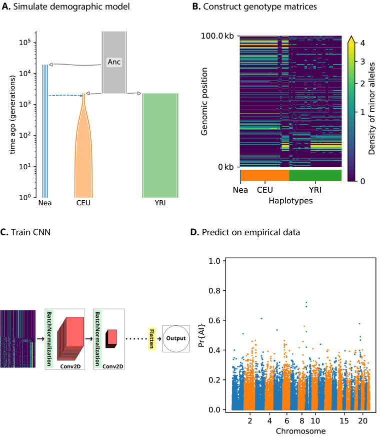
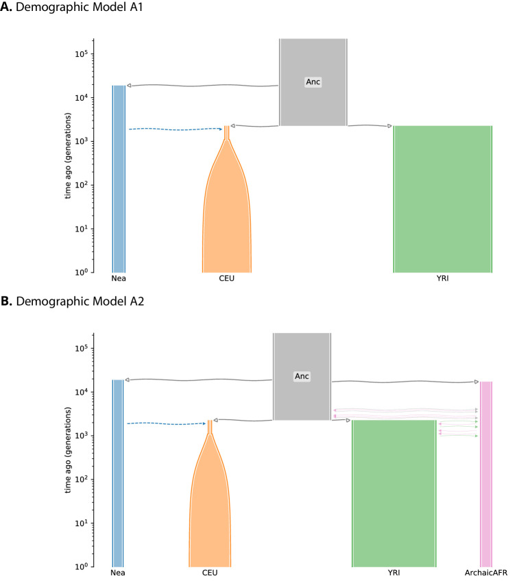
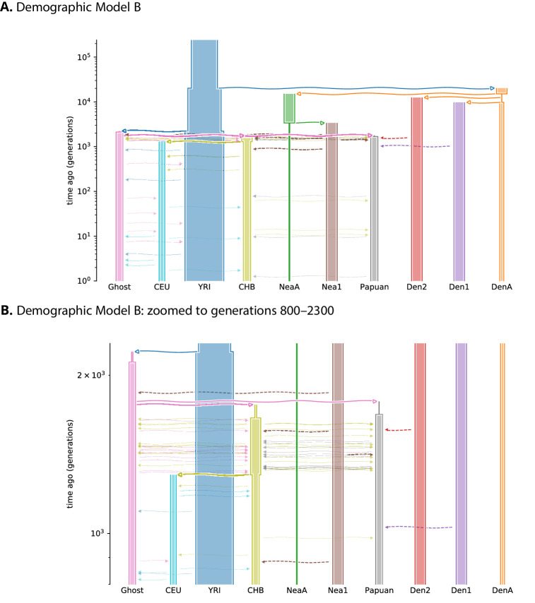
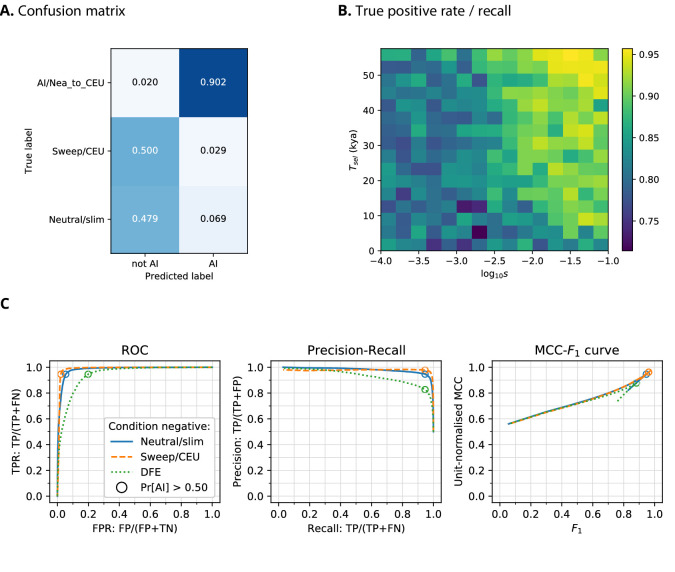
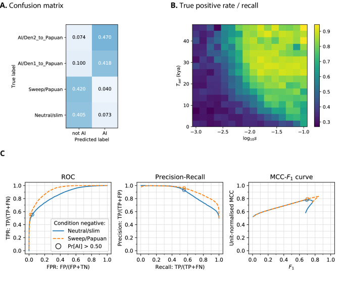
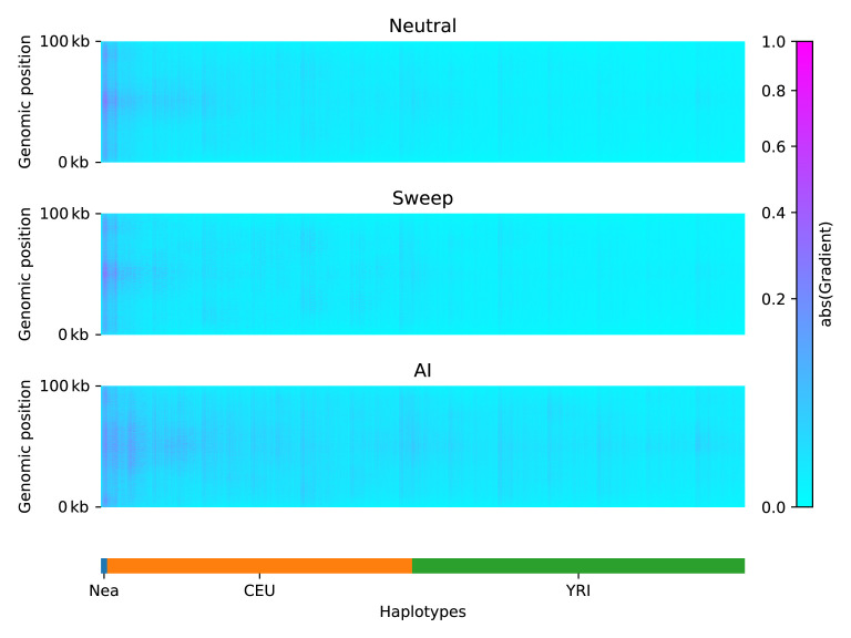
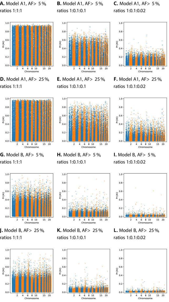
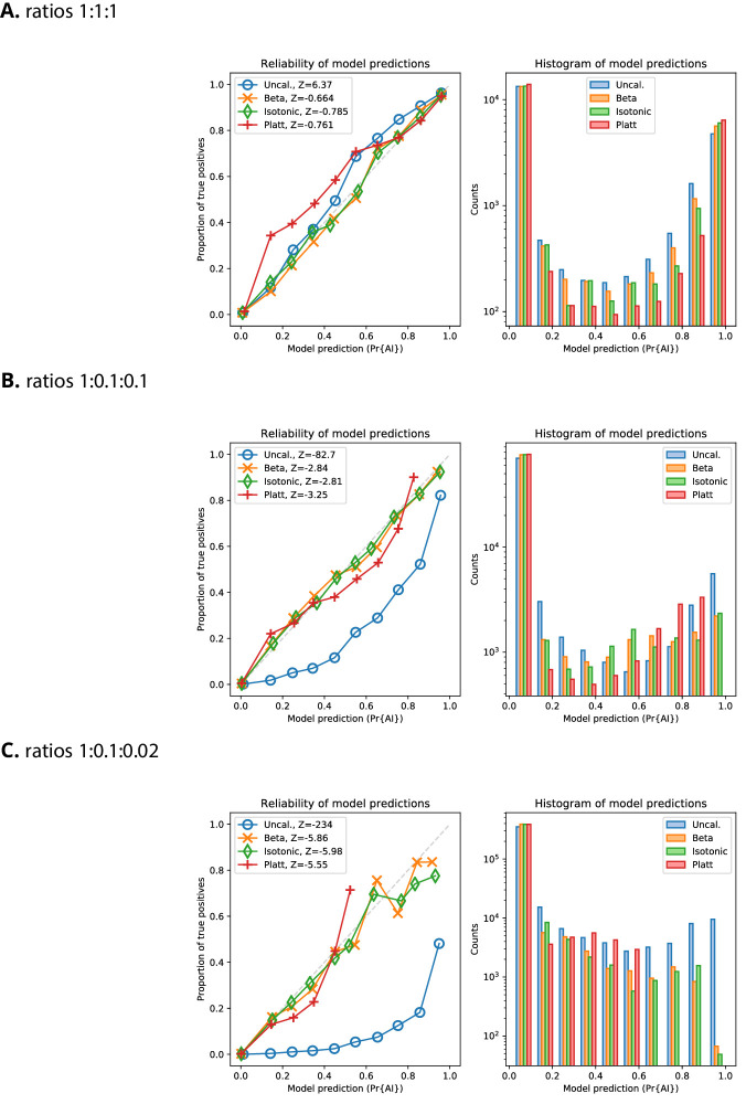
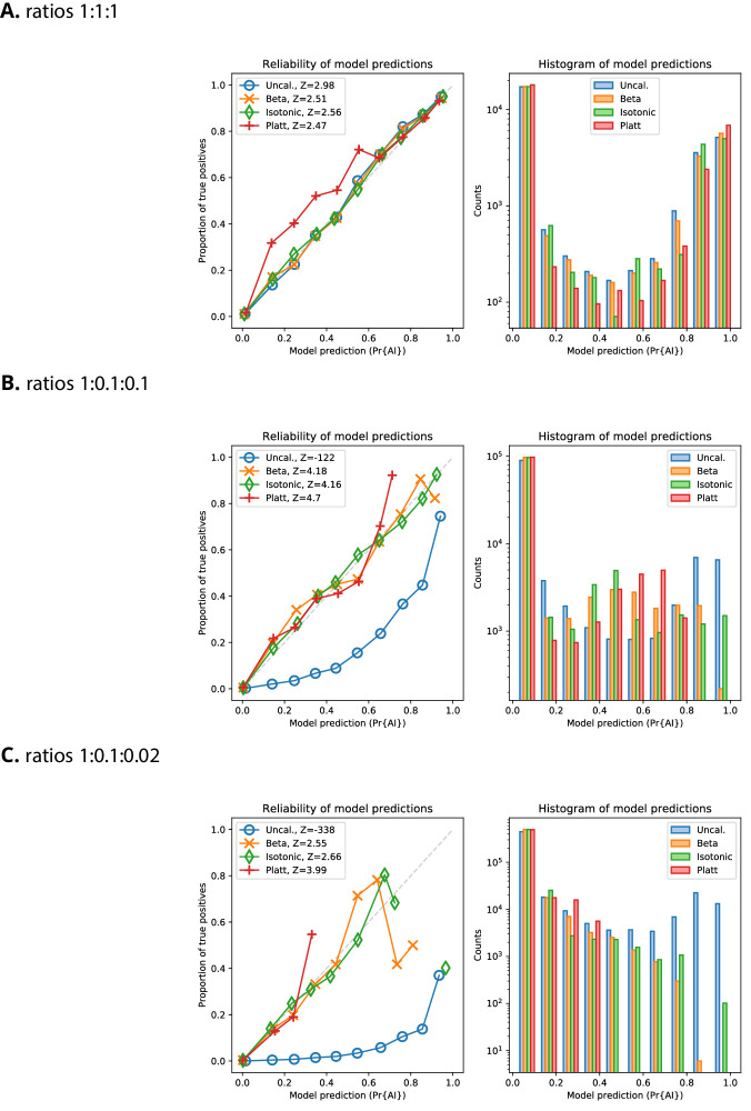
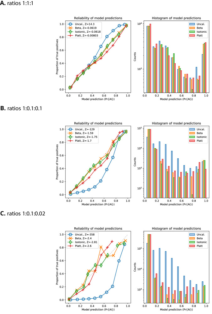
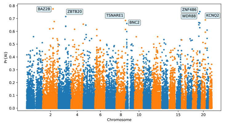
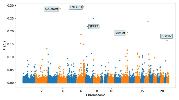
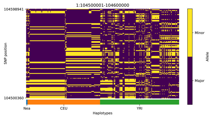
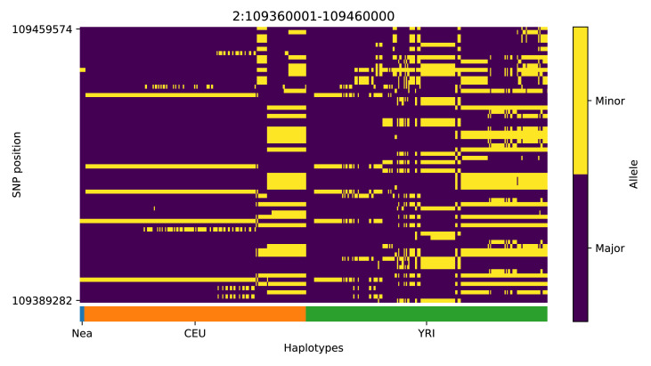
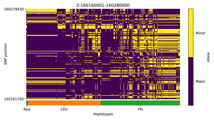
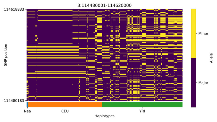
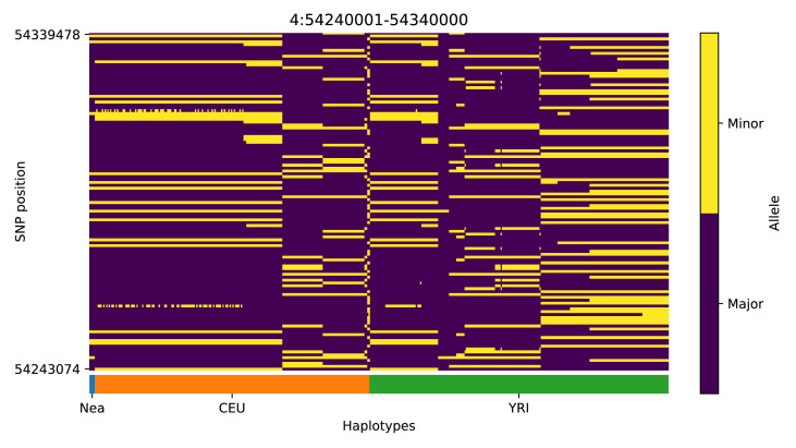
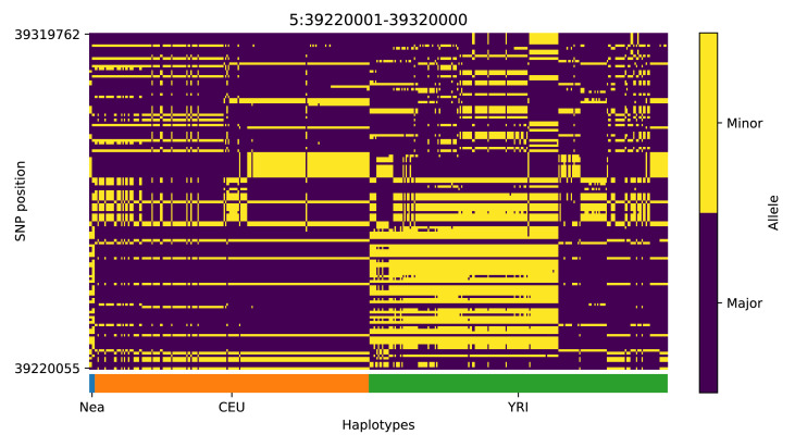
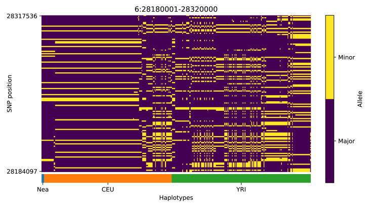
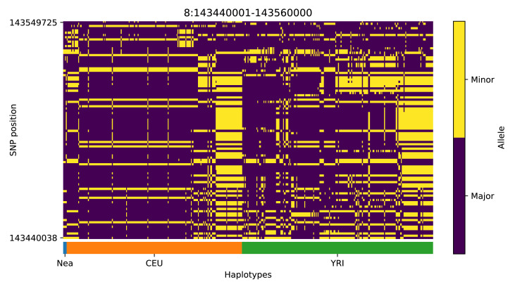
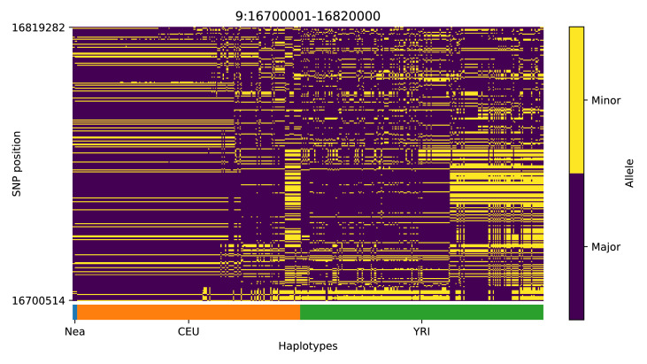
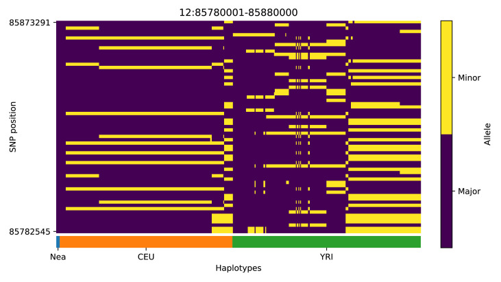
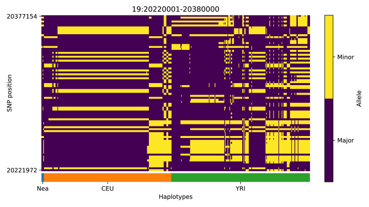
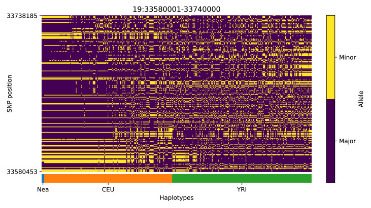
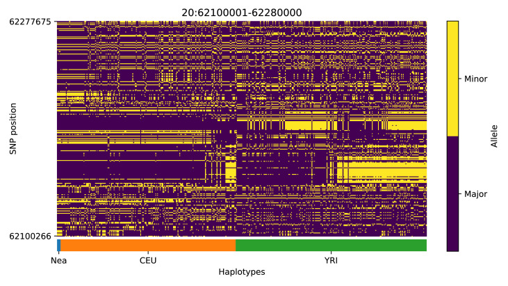
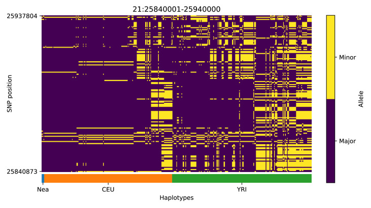
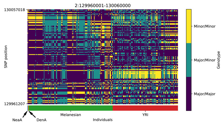
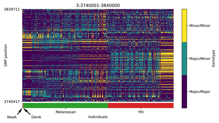
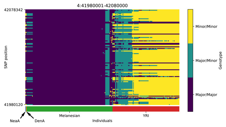
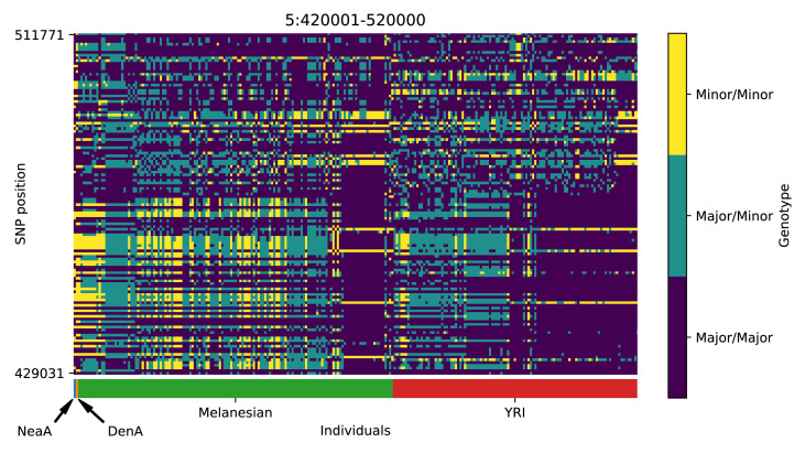
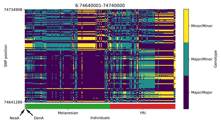
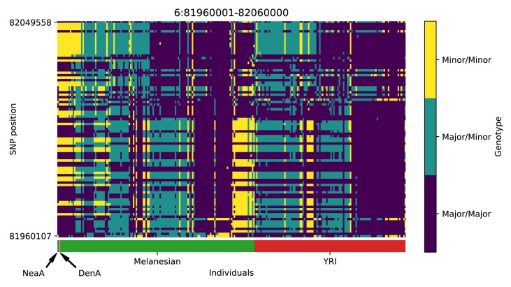
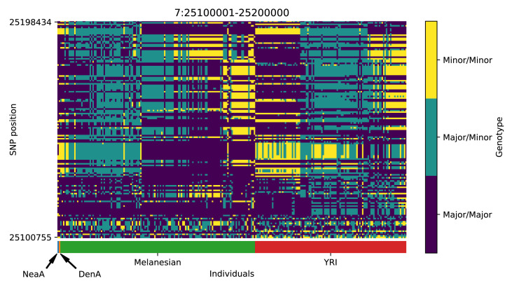
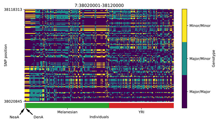
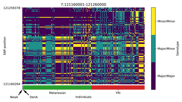
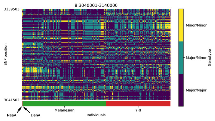
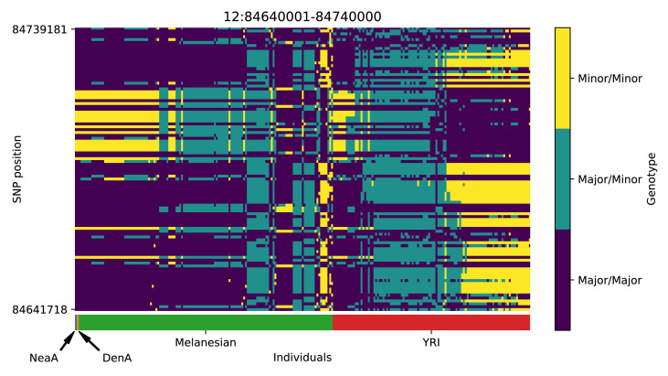
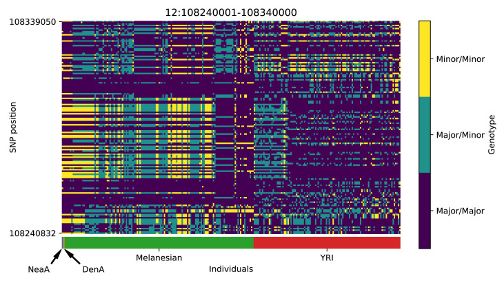
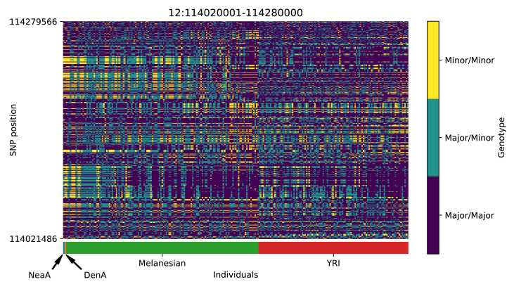
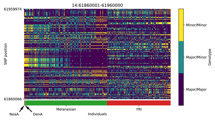
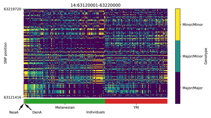
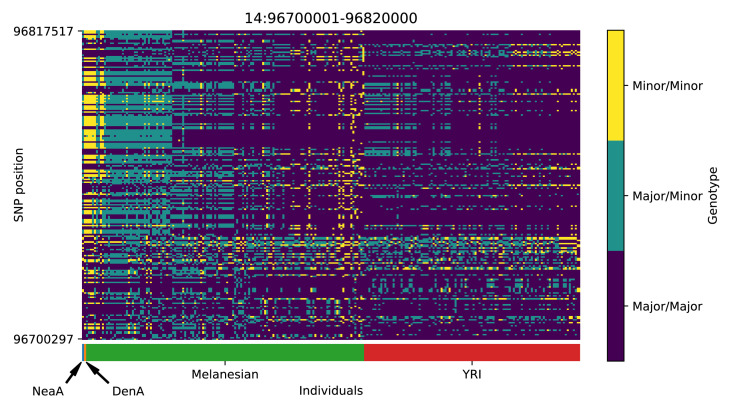
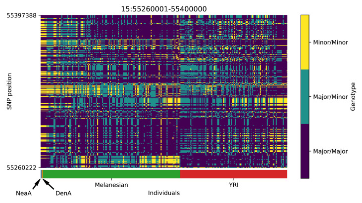
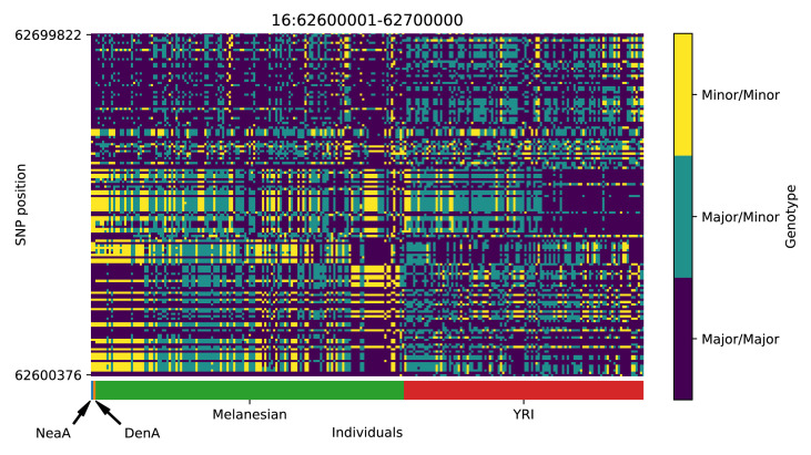
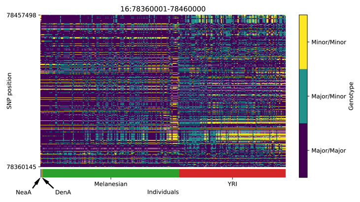
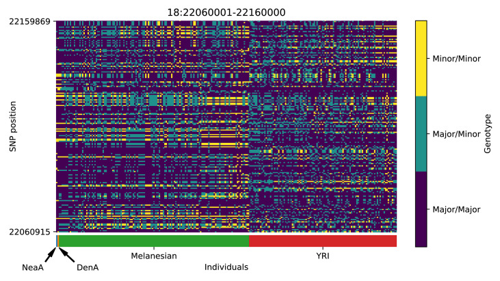
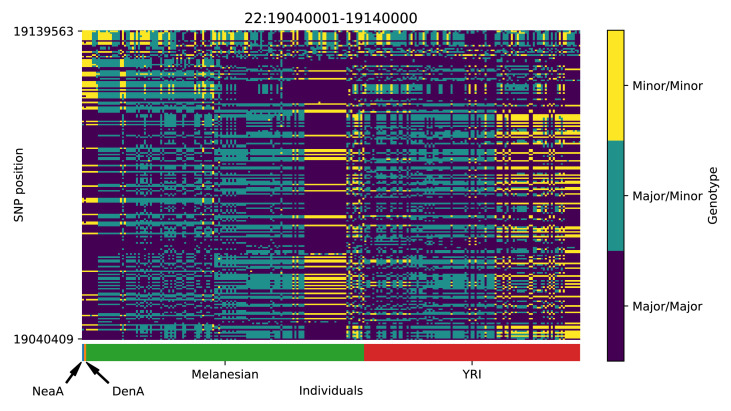
Studies in a variety of species have shown evidence for positively selected variants introduced into a population via introgression from another, distantly related population-a process known as adaptive introgression. However, there are few explicit frameworks for jointly modelling introgression and positive selection, in order to detect these variants using genomic sequence data. Here, we develop an approach based on convolutional neural networks (CNNs). CNNs do not require the specification of an analytical model of allele frequency dynamics and have outperformed alternative methods for classification and parameter estimation tasks in various areas of population genetics. Thus, they are potentially well suited to the identification of adaptive introgression. Using simulations, we trained CNNs on genotype matrices derived from genomes sampled from the donor population, the recipient population and a related non-introgressed population, in order to distinguish regions of the genome evolving under adaptive introgression from those evolving neutrally or experiencing selective sweeps. Our CNN architecture exhibits 95% accuracy on simulated data, even when the genomes are unphased, and accuracy decreases only moderately in the presence of heterosis. As a proof of concept, we applied our trained CNNs to human genomic datasets-both phased and unphased-to detect candidates for adaptive introgression that shaped our evolutionary history.

Keywords: adaptive introgression; computational biology; genetics; genomics; human; machine learning; simulation; systems biology.


Conflict of interest statement

GG, PP, MF, FR No competing interests declared

Figures

Figure 1.
Figure 1.. A schematic overview of how genomatnn detects adaptive introgression.
We first simulate a demographic history that includes introgression, such as Demographic Model A1 shown in (A), using the SLiM engine in stdpopsim. Parameter values for this model are given in Appendix 3—table 1. Three distinct scenarios are simulated for a given demographic model: neutral mutations only, a sweep in the recipient population, and adaptive introgression. The tree sequence file from each simulation is converted into a genotype matrix for input to the CNN. (B) shows a genotype matrix from an adaptive introgression simulation, where lighter pixels indicate a higher density of minor alleles, and haplotypes within each population are sorted left-to-right by similarity to the donor population (Nea). In this example, haplotype diversity is low in the recipient population (CEU), which closely resembles the donor (Nea). Thousands of simulations are produced for each simulation scenario, and their genotype matrices are used to train a binary-classification CNN (C). The CNN is trained to output Pr[AI], the probability that the input matrix corresponds to adaptive introgression. Finally, the trained CNN is applied to genotype matrices derived from a VCF/BCF file (D).
Figure 1—figure supplement 1.
Figure 1—figure supplement 1.. Schematic overview of Demographic Model A1 and A2.
Schematic overview of Demographic Model A1 (A) and A2 (B). Each population is depicted as a tube, where the tube’s width is proportional to the population’s size at any given time. Horizontal lines with arrows indicate either an ancestor/descendant relation (thick solid lines, open arrow heads), an admixture pulse (dashed lines, closed arrow heads), or a period of continuous migration (thin solid lines, closed arrow heads). The time of continuous migration lines were drawn randomly from the time interval over which the migrations occur. A Demes-format YAML file for each demographic model is available from the genomatnn git repository.
Figure 1—figure supplement 2.
Figure 1—figure supplement 2.. Schematic overview of Demographic Model B.
Overview of the Jacobs et al., 2019 demographic model (A), featuring two pulses of Denisovan gene flow into Papuans, which we implemented as the PapuansOutOfAfrica_10J19 model in stdpopsim. The same model is shown in (B), zoomed in to more clearly show the many events occurring between generations 800–2300. Each population is depicted as a tube, where the tube’s width is proportional to the population’s size at any given time. Horizontal lines with arrows indicate either an ancestor/descendant relation (thick solid lines, open arrow heads), an admixture pulse (dashed lines, closed arrow heads), or a period of continuous migration (thin solid lines, closed arrow heads). The time of continuous migration lines were drawn randomly from the time interval over which the migrations occur. DenA and NeaA are the sampled populations corresponding to Altai Denisovan and Altai Neanderthal, while Den1, Den2, and Nea1 correspond to introgressing lineages. A Demes-format YAML file for each demographic model is available from the genomatnn git repository.
Figure 2.
Figure 2.. CNN performance on validation simulations for Demographic Model A.
The CNN was trained using only AI simulations with selected mutation having allele frequency >0.25. (A) Confusion matrix. For the two prediction categories, either 'not AI' or AI, we show the proportion attributed to each of the true (simulated) scenarios. (B) Average CNN prediction for AI scenarios, binned by selection coefficient, s, and time of onset of selection Tsel. (C) ROC curves, precision-recall curves and MCC-F1 curves. The positive condition is AI. The negative conditions are shown using different line styles/colours. The circles indicate the point in ROC-space (respectively Precision-Recall-space, and MCC-F1-space) when using the threshold Pr[AI]>0.5 for classifying a genotype matrix as AI. DFE: distribution of fitness effects. TP: true positives; FP: false positives; TN: true negatives; FN: false negatives; TPR: true positive rate; FPR: false positive rate; ROC: Receiver operating characteristics; MCC: Mathews correlation coefficient; F1: harmonic mean of precision and recall.
Figure 2—figure supplement 1.
Figure 2—figure supplement 1.. Performance evaluation for Demographic Model B.
CNN performance on validation simulations for Demographic Model B with unphased data. The CNN was trained using only AI simulations with selected mutation having allele frequency > 25%. (A) Confusion matrix. For the two prediction categories, either 'not AI' or AI, we show the proportion attributed to each of the true (simulated) scenarios. (B) Average CNN prediction for AI scenarios, binned by selection coefficient, s, and time of onset of selection Tsel. (C) ROC curves, precision-recall curves and MCC-F1 curves. The positive condition is AI. The negative conditions are shown using different line styles/colours. The circles indicate the point in ROC-space (respectively Precision-Recall-space, and MCC-F1-space) when using the threshold Pr[AI]>0.5 for classifying a genotype matrix as AI. DFE: distribution of fitness effects. TP: true positives; FP: false positives; TN: true negatives; FN: false negatives; TPR: true positive rate; FPR: false positive rate; ROC: Receiver operating characteristics; MCC: Mathews correlation coefficient; F1: harmonic mean of precision and recall.
Figure 2—figure supplement 2.
Figure 2—figure supplement 2.. Comparison to other methods and performance evaluation with misspecified demographic models.
Unit-normalised Matthews correlation coefficient (MCC) versus F1 score (the harmonic mean of accuracy and precision). A value of 0.5 on the vertical axis corresponds to the performance of a random classifier. The point at coordinate (1,1) marked with a black dot corresponds to 100% true positives and 0% false negatives. Lines in MCC-F1 space were drawn by calculating the MCC and F1 values for 100 false-positive rates between 0 and 100, and the point closest to (1,1) is indicated with the symbol shown in the legend. This point may not correspond to an acceptably low false-positive rate, but for the classifiers shown here it is indicative of the method’s overall performance. In all panels, condition positive is the AI simulation scenario, and the condition negative varies by panel column (indicated at top). The 'weakly misspecified' row used simulations of Model A1 as the training/null, and evaluated the method on simulations of Model A2. The 'strongly misspecified' row used simulations of Model A1 as the training/null, and evaluated the method on simulations of Model B.
Figure 3.
Figure 3.. Saliency maps, showing the CNN’s attention across the input matrices for each simulated scenario, calculated for the CNN trained on Demographic Model A, filtered for beneficial allele frequency >0.25.
Each panel shows the average gradient over 300 input matrices encoding either neutral (top), sweep (middle), or AI (bottom) simulations. Pink/purple colours indicate larger gradients, where small changes in the genotype matrix have a relatively larger influence over the CNN’s prediction. Columns in the input matrix correspond to haplotypes from the populations labelled at the bottom.
Figure 4.
Figure 4.. Comparison of Manhattan plots using beta-calibrated output probabilities for different class ratios.
Each row indicates a single CNN, with equivalent data filtering. Each column indicates different class ratios used for calibration (Neutral:Sweep:AI). AF = Minimum beneficial allele frequency.
Figure 4—figure supplement 1.
Figure 4—figure supplement 1.. Reliability plots for Demographic Model A1 with AF > 5%.
Reliability of probabilities produced by the CNN, for the validation dataset, with and without calibration, for Demographic Model A1 with a minimum beneficial allele frequency of 5%. The variance-normalised sum of residuals is inset in the upper left corner of each of the reliability plots (Z), which for well-calibrated predictions is approximately normally distributed (Turner et al., 2019).
Figure 4—figure supplement 2.
Figure 4—figure supplement 2.. Reliability plots for Demographic Model A1 with AF > 25%.
Reliability of probabilities produced by the CNN, for the validation dataset, with and without calibration, for Demographic Model A1 with a minimum beneficial allele frequency of 25%. The variance-normalised sum of residuals is inset in the upper left corner of each of the reliability plots (Z), which for well-calibrated predictions is approximately normally distributed (Turner et al., 2019).
Figure 4—figure supplement 3.
Figure 4—figure supplement 3.. Reliability plots for Demographic Model B with AF > 5%.
Reliability of probabilities produced by the CNN, for the validation dataset, with and without calibration, for Demographic Model B with a minimum beneficial allele frequency of 5%. The variance-normalised sum of residuals is inset in the upper left corner of each of the reliability plots (Z), which for well-calibrated predictions is approximately normally distributed (Turner et al., 2019).
Figure 4—figure supplement 4.
Figure 4—figure supplement 4.. Reliability plots for Demographic Model B with AF > 25%.
Reliability of probabilities produced by the CNN, for the validation dataset, with and without calibration, for Demographic Model B with a minimum beneficial allele frequency of 25%. The variance-normalised sum of residuals is inset in the upper left corner of each of the reliability plots (Z), which for well-calibrated predictions is approximately normally distributed (Turner et al., 2019).
Figure 5.
Figure 5.. Application of the trained CNN to the Vindija and Altai Neanderthals, and 1000 genomes populations YRI and CEU.
The CNN was applied to overlapping 100 kbp windows, moving along the chromosome in steps of size 20 kbp. The CNN was trained using only AI simulations with selected mutation having allele frequency > 25%, and subsequently calibrated with resampled neutral:sweep:AI ratios of 1:0.1:0.02.
Figure 6.
Figure 6.. Application of the trained CNN to the Altai Denisovan and Altai Neanderthal, 1000 genomes YRI populations, and IGDP Melanesians.
The CNN was applied to overlapping 100 kbp windows, moving along the chromosome in steps of size 20 kbp. The CNN was trained using only AI simulations with selected mutation having allele frequency > 25%, and subsequently calibrated with resampled neutral:sweep:AI ratios of 1:0.1:0.02.
Appendix 4—figure 1.
Appendix 4—figure 1.. Haplotype plot for the candidate region chr1:104500001–104600000 in the Neanderthal-into-European AI scan.
Bright yellow indicates minor allele, dark blue indicates major allele. Haplotypes within populations are sorted left-to-right by similarity to Neanderthals.
Appendix 4—figure 2.
Appendix 4—figure 2.. Haplotype plot for the candidate region chr2:109360001–109460000 in the Neanderthal-into-European AI scan.
Bright yellow indicates minor allele, dark blue indicates major allele. Haplotypes within populations are sorted left-to-right by similarity to Neanderthals.
Appendix 4—figure 3.
Appendix 4—figure 3.. Haplotype plot for the candidate region chr2:160160001–160280000 in the Neanderthal-into-European AI scan.
Bright yellow indicates minor allele, dark blue indicates major allele. Haplotypes within populations are sorted left-to-right by similarity to Neanderthals.
Appendix 4—figure 4.
Appendix 4—figure 4.. Haplotype plot for the candidate region chr3:114480001–114620000 in the Neanderthal-into-European AI scan.
Bright yellow indicates minor allele, dark blue indicates major allele. Haplotypes within populations are sorted left-to-right by similarity to Neanderthals.
Appendix 4—figure 5.
Appendix 4—figure 5.. Haplotype plot for the candidate region chr4:54240001–54340000 in the Neanderthal-into-European AI scan.
Bright yellow indicates minor allele, dark blue indicates major allele. Haplotypes within populations are sorted left-to-right by similarity to Neanderthals.
Appendix 4—figure 6.
Appendix 4—figure 6.. Haplotype plot for the candidate region chr5:39220001–39320000 in the Neanderthal-into-European AI scan.
Bright yellow indicates minor allele, dark blue indicates major allele. Haplotypes within populations are sorted left-to-right by similarity to Neanderthals.
Appendix 4—figure 7.
Appendix 4—figure 7.. Haplotype plot for the candidate region chr6:28180001–28320000 in the Neanderthal-into-European AI scan.
Bright yellow indicates minor allele, dark blue indicates major allele. Haplotypes within populations are sorted left-to-right by similarity to Neanderthals.
Appendix 4—figure 8.
Appendix 4—figure 8.. Haplotype plot for the candidate region chr8:143440001–143560000 in the Neanderthal-into-European AI scan.
Bright yellow indicates minor allele, dark blue indicates major allele. Haplotypes within populations are sorted left-to-right by similarity to Neanderthals.
Appendix 4—figure 9.
Appendix 4—figure 9.. Haplotype plot for the candidate region chr9:16700001–16820000 in the Neanderthal-into-European AI scan.
Bright yellow indicates minor allele, dark blue indicates major allele. Haplotypes within populations are sorted left-to-right by similarity to Neanderthals.
Appendix 4—figure 10.
Appendix 4—figure 10.. Haplotype plot for the candidate region chr12:85780001–85880000 in the Neanderthal-into-European AI scan.
Bright yellow indicates minor allele, dark blue indicates major allele. Haplotypes within populations are sorted left-to-right by similarity to Neanderthals.
Appendix 4—figure 11.
Appendix 4—figure 11.. Haplotype plot for the candidate region chr19:20220001–20380000 in the Neanderthal-into-European AI scan.
Bright yellow indicates minor allele, dark blue indicates major allele. Haplotypes within populations are sorted left-to-right by similarity to Neanderthals.
Appendix 4—figure 12.
Appendix 4—figure 12.. Haplotype plot for the candidate region chr19:33580001–33740000 in the Neanderthal-into-European AI scan.
Bright yellow indicates minor allele, dark blue indicates major allele. Haplotypes within populations are sorted left-to-right by similarity to Neanderthals.
Appendix 4—figure 13.
Appendix 4—figure 13.. Haplotype plot for the candidate region chr20:62100001–62280000 in the Neanderthal-into-European AI scan.
Bright yellow indicates minor allele, dark blue indicates major allele. Haplotypes within populations are sorted left-to-right by similarity to Neanderthals.
Appendix 4—figure 14.
Appendix 4—figure 14.. Haplotype plot for the candidate region chr21:25840001–25940000 in the Neanderthal-into-European AI scan.
Bright yellow indicates minor allele, dark blue indicates major allele. Haplotypes within populations are sorted left-to-right by similarity to Neanderthals.
Appendix 5—figure 1.
Appendix 5—figure 1.. Genotype plot for the candidate region chr2:129960001–130060000 in the Denisovan-into-Melanesian AI scan.
Dark blue = homozygote major allele, light blue = heterozygote, yellow = homozygote minor allele. Genotypes within populations are sorted left-to-right by similarity to the Denisovan.
Appendix 5—figure 2.
Appendix 5—figure 2.. Genotype plot for the candidate region chr3:3740001–3840000 in the Denisovan-into-Melanesian AI scan.
Dark blue = homozygote major allele, light blue = heterozygote, yellow = homozygote minor allele. Genotypes within populations are sorted left-to-right by similarity to the Denisovan.
Appendix 5—figure 3.
Appendix 5—figure 3.. Genotype plot for the candidate region chr4:41980001–42080000 in the Denisovan-into-Melanesian AI scan.
Dark blue = homozygote major allele, light blue = heterozygote, yellow = homozygote minor allele. Genotypes within populations are sorted left-to-right by similarity to the Denisovan.
Appendix 5—figure 4.
Appendix 5—figure 4.. Genotype plot for the candidate region chr5:420001–520000 in the Denisovan-into-Melanesian AI scan.
Dark blue = homozygote major allele, light blue = heterozygote, yellow = homozygote minor allele. Genotypes within populations are sorted left-to-right by similarity to the Denisovan.
Appendix 5—figure 5.
Appendix 5—figure 5.. Genotype plot for the candidate region chr6:74640001–74740000 in the Denisovan-into-Melanesian AI scan.
Dark blue = homozygote major allele, light blue = heterozygote, yellow = homozygote minor allele. Genotypes within populations are sorted left-to-right by similarity to the Denisovan.
Appendix 5—figure 6.
Appendix 5—figure 6.. Genotype plot for the candidate region chr6:81960001–82060000 in the Denisovan-into-Melanesian AI scan.
Dark blue = homozygote major allele, light blue = heterozygote, yellow = homozygote minor allele. Genotypes within populations are sorted left-to-right by similarity to the Denisovan.
Appendix 5—figure 7.
Appendix 5—figure 7.. Genotype plot for the candidate region chr6:137920001–138120000 in the Denisovan-into-Melanesian AI scan.
Dark blue = homozygote major allele, light blue = heterozygote, yellow = homozygote minor allele. Genotypes within populations are sorted left-to-right by similarity to the Denisovan.
Appendix 5—figure 8.
Appendix 5—figure 8.. Genotype plot for the candidate region chr7:25100001–25200000 in the Denisovan-into-Melanesian AI scan.
Dark blue = homozygote major allele, light blue = heterozygote, yellow = homozygote minor allele. Genotypes within populations are sorted left-to-right by similarity to the Denisovan.
Appendix 5—figure 9.
Appendix 5—figure 9.. Genotype plot for the candidate region chr7:38020001–38120000 in the Denisovan-into-Melanesian AI scan.
Dark blue = homozygote major allele, light blue = heterozygote, yellow = homozygote minor allele. Genotypes within populations are sorted left-to-right by similarity to the Denisovan.
Appendix 5—figure 10.
Appendix 5—figure 10.. Genotype plot for the candidate region chr7:121160001–121260000 in the Denisovan-into-Melanesian AI scan.
Dark blue = homozygote major allele, light blue = heterozygote, yellow = homozygote minor allele. Genotypes within populations are sorted left-to-right by similarity to the Denisovan.
Appendix 5—figure 11.
Appendix 5—figure 11.. Genotype plot for the candidate region chr8:3040001–3140000 in the Denisovan-into-Melanesian AI scan.
Dark blue = homozygote major allele, light blue = heterozygote, yellow = homozygote minor allele. Genotypes within populations are sorted left-to-right by similarity to the Denisovan.
Appendix 5—figure 12.
Appendix 5—figure 12.. Genotype plot for the candidate region chr12:84640001–84740000 in the Denisovan-into-Melanesian AI scan.
Dark blue = homozygote major allele, light blue = heterozygote, yellow = homozygote minor allele. Genotypes within populations are sorted left-to-right by similarity to the Denisovan.
Appendix 5—figure 13.
Appendix 5—figure 13.. Genotype plot for the candidate region chr12:108240001–108340000 in the Denisovan-into-Melanesian AI scan.
Dark blue = homozygote major allele, light blue = heterozygote, yellow = homozygote minor allele. Genotypes within populations are sorted left-to-right by similarity to the Denisovan.
Appendix 5—figure 14.
Appendix 5—figure 14.. Genotype plot for the candidate region chr12:114020001–114280000 in the Denisovan-into-Melanesian AI scan.
Dark blue = homozygote major allele, light blue = heterozygote, yellow = homozygote minor allele. Genotypes within populations are sorted left-to-right by similarity to the Denisovan.
Appendix 5—figure 15.
Appendix 5—figure 15.. Genotype plot for the candidate region chr14:61860001–61960000 in the Denisovan-into-Melanesian AI scan.
Dark blue = homozygote major allele, light blue = heterozygote, yellow = homozygote minor allele. Genotypes within populations are sorted left-to-right by similarity to the Denisovan.
Appendix 5—figure 16.
Appendix 5—figure 16.. Genotype plot for the candidate region chr14:63120001–63220000 in the Denisovan-into-Melanesian AI scan.
Dark blue = homozygote major allele, light blue = heterozygote, yellow = homozygote minor allele. Genotypes within populations are sorted left-to-right by similarity to the Denisovan.
Appendix 5—figure 17.
Appendix 5—figure 17.. Genotype plot for the candidate region chr14:96700001–96820000 in the Denisovan-into-Melanesian AI scan.
Dark blue = homozygote major allele, light blue = heterozygote, yellow = homozygote minor allele. Genotypes within populations are sorted left-to-right by similarity to the Denisovan.
Appendix 5—figure 18.
Appendix 5—figure 18.. Genotype plot for the candidate region chr15:55260001–55400000 in the Denisovan-into-Melanesian AI scan.
Dark blue = homozygote major allele, light blue = heterozygote, yellow = homozygote minor allele. Genotypes within populations are sorted left-to-right by similarity to the Denisovan.
Appendix 5—figure 19.
Appendix 5—figure 19.. Genotype plot for the candidate region chr16:62600001–62700000 in the Denisovan-into-Melanesian AI scan.
Dark blue = homozygote major allele, light blue = heterozygote, yellow = homozygote minor allele. Genotypes within populations are sorted left-to-right by similarity to the Denisovan.
Appendix 5—figure 20.
Appendix 5—figure 20.. Genotype plot for the candidate region chr16:78360001–78460000 in the Denisovan-into-Melanesian AI scan.
Dark blue = homozygote major allele, light blue = heterozygote, yellow = homozygote minor allele. Genotypes within populations are sorted left-to-right by similarity to the Denisovan.
Appendix 5—figure 21.
Appendix 5—figure 21.. Genotype plot for the candidate region chr18:22060001–22160000 in the Denisovan-into-Melanesian AI scan.
Dark blue = homozygote major allele, light blue = heterozygote, yellow = homozygote minor allele. Genotypes within populations are sorted left-to-right by similarity to the Denisovan.
Appendix 5—figure 22.
Appendix 5—figure 22.. Genotype plot for the candidate region chr22:19040001–19140000 in the Denisovan-into-Melanesian AI scan.
Dark blue = homozygote major allele, light blue = heterozygote, yellow = homozygote minor allele. Genotypes within populations are sorted left-to-right by similarity to the Denisovan.

References

    1. Abadi M, Agarwal A, Barham P, Brevdo E, Chen Z, Citro C, Corrado GS, Davis A, Dean J, Devin M, Ghemawat S, Goodfellow I, Harp A, Irving G, Isard M, Jia Y, Jozefowicz R, Kaiser L, Kudlur M, Levenberg J, Mané D, Monga R, Moore S, Murray D, Olah C, Schuster M, Shlens J, Steiner B, Sutskever I, Talwar K, Tucker P, Vanhoucke V, Vasudevan V, Viégas F, Vinyals O, Warden P, Wattenberg M, Wicke M, Yu Y, Zheng X. TensorFlow: large-scale machine learning on heterogeneous systems. arXiv. 2015 https://arxiv.org/abs/1603.04467
    1. Adrion JR, Cole CB, Dukler N, Galloway JG, Gladstein AL, Gower G, Kyriazis CC, Ragsdale AP, Tsambos G, Baumdicker F, Carlson J, Cartwright RA, Durvasula A, Gronau I, Kim BY, McKenzie P, Messer PW, Noskova E, Ortega-Del Vecchyo D, Racimo F, Struck TJ, Gravel S, Gutenkunst RN, Lohmueller KE, Ralph PL, Schrider DR, Siepel A, Kelleher J, Kern AD. A community-maintained standard library of population genetic models. eLife. 2020a;9:e54967. doi: 10.7554/eLife.54967. - DOI - PMC - PubMed
    1. Adrion JR, Galloway JG, Kern AD. Predicting the landscape of recombination using deep learning. Molecular Biology and Evolution. 2020b;37:1790–1808. doi: 10.1093/molbev/msaa038. - DOI - PMC - PubMed
    1. Aggarwal CC. Neural Networks and Deep Learning. Springer; 2018. - DOI
    1. Alaa AM, van der Schaar M. Demystifying black-box models with symbolic metamodels. In: Wallach H, Larochelle H, Beygelzimer A, Alché-Buc F. d, Fox E, Garnett R, editors. Advances in Neural Information Processing Systems 32. Curran Associates, Inc; 2019. pp. 11304–11314.

Publication types