AutoStepfinder: A fast and automated step detection method for single-molecule analysis

Abstract

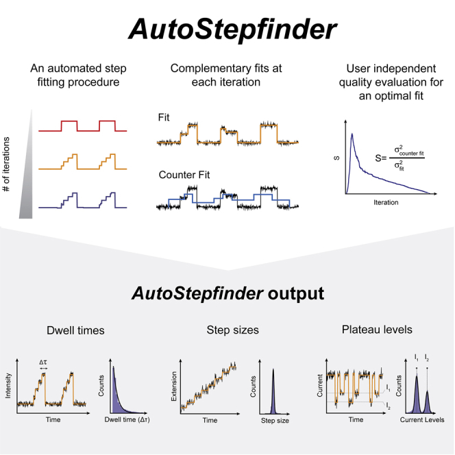
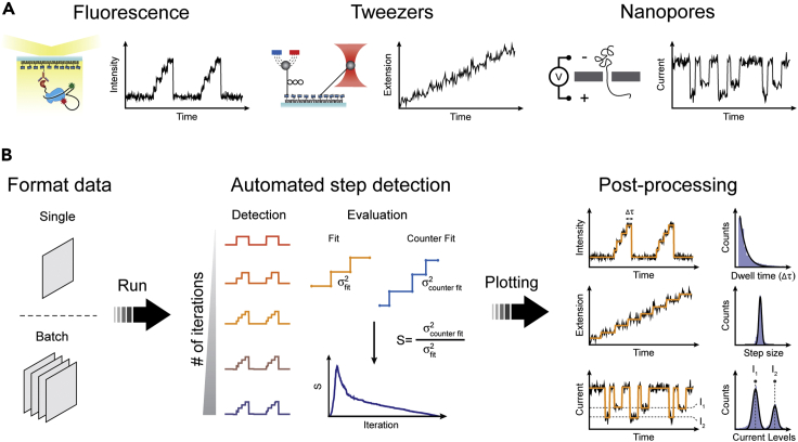
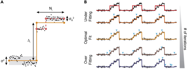
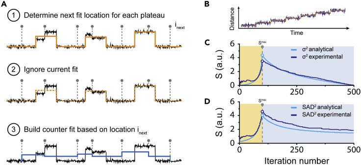
Single-molecule techniques allow the visualization of the molecular dynamics of nucleic acids and proteins with high spatiotemporal resolution. Valuable kinetic information of biomolecules can be obtained when the discrete states within single-molecule time trajectories are determined. Here, we present a fast, automated, and bias-free step detection method, AutoStepfinder, that determines steps in large datasets without requiring prior knowledge on the noise contributions and location of steps. The analysis is based on a series of partition events that minimize the difference between the data and the fit. A dual-pass strategy determines the optimal fit and allows AutoStepfinder to detect steps of a wide variety of sizes. We demonstrate step detection for a broad variety of experimental traces. The user-friendly interface and the automated detection of AutoStepfinder provides a robust analysis procedure that enables anyone without programming knowledge to generate step fits and informative plots in less than an hour.

Keywords: AutoStepfinder; Stepfinder; biophysics; data analysis; fluorescence; magnetic tweezer; nanopore; optical tweezer; single molecule; step detection.

Graphical abstract

Figure 1

Workflow of AutoStepfinder (A) AutoStepfinder can be applied on a wide variety single-molecule of trajectories, including single-molecule fluorescence, magnetic and optical tweezers, and nanopore data. (B) The algorithm requires input in the form of one or multiple.txt files with one or two columns (signal value or time and signal value). After pressing run, the algorithm iteratively adds single steps to the data that minimizes the σ² value. For each iteration, the quality is assessed by means of a secondary counter fit. Finally, the best fit is selected and the algorithm outputs the corresponding fit, dwell times, step sizes, and levels. Fitting large datasets (>10⁶ data points) can be done in less than 1 min with a desktop computer. Also see Figure S1.

Figure 2

Global arrangement of the AutoStepfinder algorithm (A) An example of an iterative step fit (orange line) on a single-molecule trajectory (black dots). Single-molecule trajectories are fitted by the AutoStepfinder algorithm by iteratively minimizing the σ² value. To perform a step fit the program assumes that the data contain steps (Δ_i), bounded by a plateau (N_i) that is subject to residual noise (σ_R², gray box). After the first step fit, AutoStepfinder selects the plateau with the largest value of σ², for the next partition event (red dashed lines). This process continues until the maximum number of iterations is reached. (B) An example of the iterative process of step fitting by the AutoStepfinder algorithm. The algorithm successively adds a single step to the data (cyan triangles) and thereby minimizes the σ² value. Step fitting below the optimal number of steps is considered underfitting, whereas step fitting beyond the optimal number of steps is considered overfitting. Also see Figure S1.

Figure 3

Determining the quality of a step fit (A) For every step fit the algorithm performs, the quality of the fit (orange line) is evaluated by means of an additional fit (blue line, called a counter fit). The counter fit is built by determining the next partition point (i_next), after which the current is rejected. Subsequently, the algorithm places the counter fit (blue) plateaus at locations within the existing fit (orange). (B) Simulated trajectory representing a motor stepping behavior. (C) Representative example of experimental and analytical S-curves obtained by fitting the trajectory in (B) through minimization of σ². Shaded areas indicate the underfitting (yellow) and overfitting (light blue) regime. (D) Representative example of experimental and analytical S-curves obtained by fitting the trajectory in (B) through minimization of the sum of absolute differences (SAD²). Shaded areas indicate the underfitting (yellow) and overfitting (light blue) regime. Also see Figure S2.

Figure 4

Dual-pass step detection to detect a wide range of step sizes (A) A simulated single-molecule trajectory displaying uniform steps with a size of Δ1. (B) An example trace displaying uniform steps with a size of Δ₂. (C) A simulated single-molecule trajectory displaying non-uniform steps with a size of Δ_1’ and Δ_2’. (D) S-curves for the three example traces displayed in (A–C). The global maximums of peak 1 (S_P1^max) and peak 2 (S_P2^max) are indicated with dashed gray lines. The S-curve for the dataset with both large (Δ₁) and small (Δ₂) steps exhibits two peaks.

Figure 5

Testing the detection limits of AutoStepfinder (A) Simulated time trajectories that were exposed to various noise levels to benchmark the AutoStepfinder algorithm. The data start with a step of 10 arbitrary units (a.u.), the subsequent steps decrease by 1 a.u. until the smallest step size of 1 a.u. is reached. This idealized trajectory was repeated 100 times, resulting in a dataset in which each step size occurred 100 times. (B) Distribution of step sizes of the simulated trajectories, obtained through the AutoStepfinder algorithm. The red dashed lines indicate the position of each bin when 100% of the steps are correctly identified. C) Schematic of the step injection test. To quantify the probability that AutoStepfinder would detect steps with a certain size (Δ_inject), steps were injected (pink curve, middle) into an existing trajectory (blue curve, top) to generate a benchmark curve (orange curve, bottom). (D) Histogram of the detection probability of step sizes at various noise levels (SD). Solid lines represent sigmoidal fits to the data. (E) Histogram showing the distribution of the 95% confidence intervals of the step sizes (cyan bars) obtained by bootstrap analysis. The line (purple) indicates the deviation of the fit from the ground truth. (F) Histogram showing the distribution of the 95% confidence intervals of the plateaus lengths (cyan bars) obtained by bootstrap analysis. The line (purple) indicates the deviation of the fit from the ground truth. (G) Relation between the SNR and the error in the determined steps. (H) Relation between the SNR and the error in the determined plateaus (cyan line). The purple line indicates the deviation between the final fit and a local refit at various noise levels (iteration error). Also see Figure S4.

Figure 6

Comparison of AutoStepfinder with other methods (A) Examples of simulated single-molecule trajectories that were exposed to distinct noise types, each with an SD of 2.0. The noise types are Gaussian noise (purple), Poissonian noise (orange), correlated noise (pink), and humming noise (light blue). (B) Step detection by a Schwarz information criterion (SIC)-based algorithm. For each step fit, the quality of the fit is evaluated by calculating an SIC score. The SIC curve displays a minimum when the optimal fit is reached (circle). The dashed gray line indicates the number of steps in the data. Notably, the SIC curve of Gaussian noise (purple) overlaps the SIC curve of the Poissonian noise (orange). (C) Step detection by the AutoStepfinder algorithm. For each step fit, the quality of the fit is evaluated by performing an additional fit, called counter fit, and calculating an S-score. The S-curve displays a maximum when the optimal fit is reached (circle). The dashed gray line indicates the number of steps in the data. (D) Performance of the AutoStepfinder algorithm and SIC-based algorithm on simulated single-molecule trajectories that were exposed to distinct noise types with SD = 2.0. A more extensive overview on the robustness of AutoStepfinder- and the SIC-based algorithms is provided in Figure S4. (E) Examples of simulated single-molecule trajectories each with a distinct number of states (gray). The purple, orange, and cyan lines indicate the ground truth, states found by AutoStepfinder, and the states found by iHMM, respectively. The displayed trajectories were exposed to Gaussian noise with an SNR of 1.0. (F) Comparison of AutoStepfinder (orange) and iHMM (cyan). The size of the circles indicates the percentage states that were within a distance of 25% of a step size of the ground truth. The circles in gray indicate the percentage scale. Also see Figure S5.

Figure 7

Application of AutoStepfinder on experimental FRET data (A) Schematic of loop formation by the CRISPR-associated Cas3 helicase/nuclease protein (blue). The appearance of FRET during loop formation is indicated by the size of the star: low FRET, large green star, or high FRET, large red star. (B) A representative FRET trace (dark blue) fitted with the AutoStepfinder algorithm (orange). (C) S-curve for the first round of fitting by AutoStepfinder. The dashed gray line indicates the S_P1^max of the S-curve. (D) S-curve for the second round of fitting by AutoStepfinder. The global maximum of the S-curve for the second round was below the set acceptance threshold and therefore the second round of fitting was not executed. (E) Distribution of FRET levels obtained through the AutoStepfinder algorithm. Black lines represent a Gaussian fit. (F) Distribution of step sizes obtained through the AutoStepfinder algorithm. Data were fitted with a gamma distribution (solid line) to obtain the number of hidden steps (n) and rate (k). Error represents the 95% confidence interval obtained through bootstrap analysis. (G) Dwell time distribution obtained through the AutoStepfinder algorithm. Black lines represent a gamma distribution. Also see Figure S6.

References

1. Juette M.F., Terry D.S., Wasserman M.R., Zhou Z., Altman R.B., Zheng Q., Blanchard S.C. The bright future of single-molecule fluorescence imaging. Curr. Opin. Chem. Biol. 2014;20:103–111. - PMC - PubMed
1. Ha T. Single-molecule methods leap ahead. Nat. Methods. 2014;11:1015–1018. - PubMed
1. Forties R.A., Wang M.D. Minireview discovering the power of single molecules. Cell. 2014;157:4–7. - PubMed
1. Joo C., Fareh M., Narry Kim V. Bringing single-molecule spectroscopy to macromolecular protein complexes. Trends Biochem. Sci. 2013;38:30–37. - PMC - PubMed
1. Svoboda K., Schmidt C.F., Schnapp B.J., Block S.M. Direct observation of kinesin stepping by optical trapping interferometry. Nature. 1993;365:721–727. - PubMed