Embedding optimization reveals long-lasting history dependence in neural spiking activity

Abstract

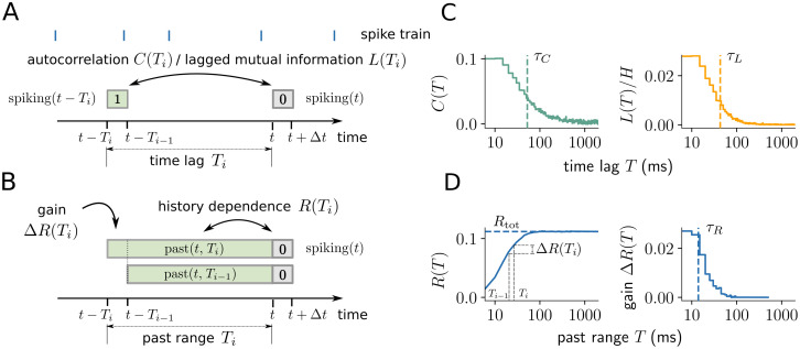
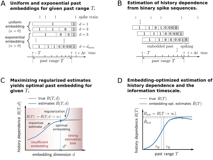
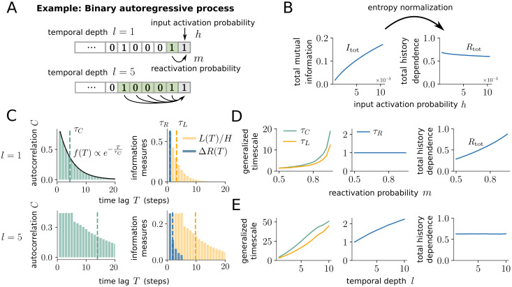
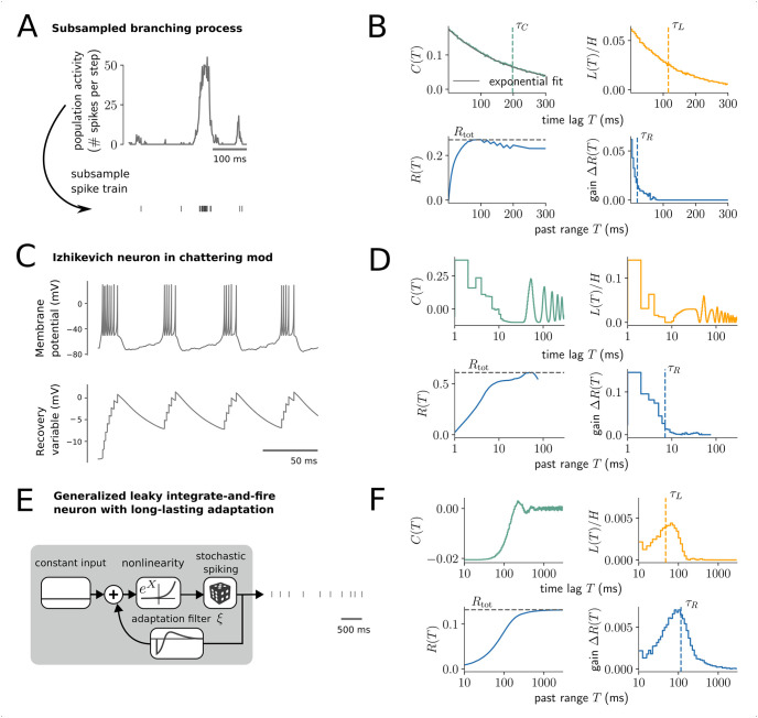
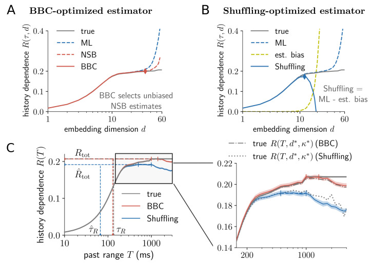
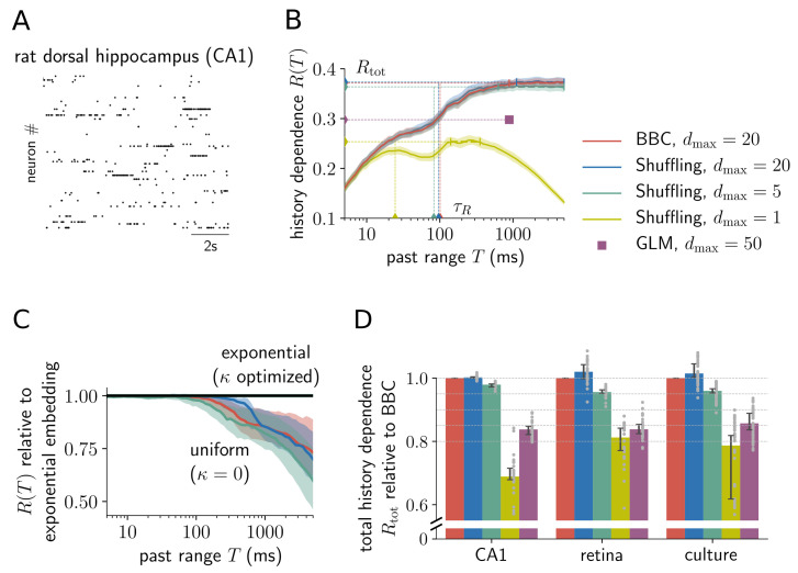
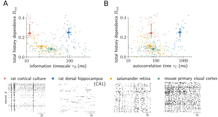
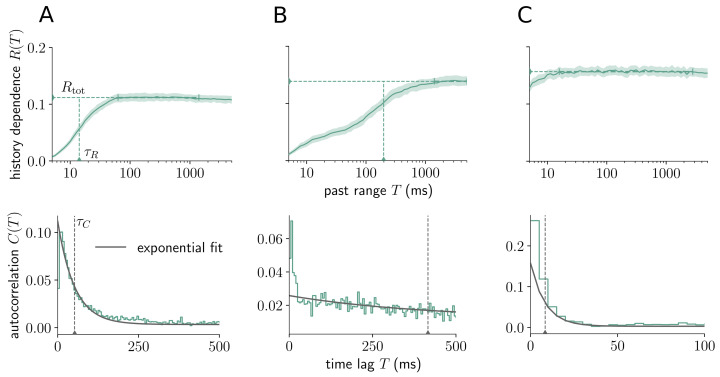
Information processing can leave distinct footprints on the statistics of neural spiking. For example, efficient coding minimizes the statistical dependencies on the spiking history, while temporal integration of information may require the maintenance of information over different timescales. To investigate these footprints, we developed a novel approach to quantify history dependence within the spiking of a single neuron, using the mutual information between the entire past and current spiking. This measure captures how much past information is necessary to predict current spiking. In contrast, classical time-lagged measures of temporal dependence like the autocorrelation capture how long-potentially redundant-past information can still be read out. Strikingly, we find for model neurons that our method disentangles the strength and timescale of history dependence, whereas the two are mixed in classical approaches. When applying the method to experimental data, which are necessarily of limited size, a reliable estimation of mutual information is only possible for a coarse temporal binning of past spiking, a so-called past embedding. To still account for the vastly different spiking statistics and potentially long history dependence of living neurons, we developed an embedding-optimization approach that does not only vary the number and size, but also an exponential stretching of past bins. For extra-cellular spike recordings, we found that the strength and timescale of history dependence indeed can vary independently across experimental preparations. While hippocampus indicated strong and long history dependence, in visual cortex it was weak and short, while in vitro the history dependence was strong but short. This work enables an information-theoretic characterization of history dependence in recorded spike trains, which captures a footprint of information processing that is beyond time-lagged measures of temporal dependence. To facilitate the application of the method, we provide practical guidelines and a toolbox.

Fig 1. Illustration of history dependence and related measures in a neural spike train.

(A) For the analysis, spiking is represented by 0 or 1 in a small time bin Δt (grey box). Autocorrelation C(T_i) or the lagged mutual information L(T_i) quantify the statistical dependence of spiking on past spiking in a single past bin with time lag T_i (green box). (B) In contrast, history dependence R(T_i) quantifies the dependence of spiking on the entire spiking history in a past range T_i. The gain in history dependence ΔR(T_i) = R(T_i) − R(T_i−1) quantifies the increase in history dependence by increasing the past range from T_i−1 to T_i, and is defined in analogy to the lagged measures. (C) Autocorrelation C(T) and lagged mutual information L(T) for a typical example neuron (mouse, primary visual cortex). Both measures decay with increasing T, where L(T) decays slightly faster due to the non-linearity of the mutual information. Timescales τ_C and τ_L (vertical dashed lines) can be computed either by fitting an exponential decay (autocorrelation) or by using the generalized timescale (lagged mutual information). (D) In contrast, history dependence R(T) increases monotonically for systematically increasing past range T, until it saturates at the total history dependence R_tot. From R(T), the gain ΔR(T_i) can be computed between increasing past ranges T_i−1 and T_i (grey dashed lines). The gain ΔR(T) decays to zero like the time-lagged measures, with information timescale τ_R (dashed line).

Fig 2. Illustration of embedding optimization to estimate history dependence and the information timescale.

(A) History dependence R is estimated from the observed joint statistics of current spiking in a small time bin [t + Δt) (dark grey) and the embedded past, i.e. a binary sequence representing past spiking in a past window [t − T, t). We systematically vary the number of bins d and bin sizes for fixed past range T. Bin sizes scale exponentially with bin index and a scaling exponent κ to reduce resolution for spikes farther into the past. (B) The joint statistics of current and past spiking are obtained by shifting the past range in steps of Δt and counting the resulting binary sequences. (C) Finding a good choice of embedding parameters (e.g. embedding dimension d) is challenging: When d is chosen too small, the true history dependence R(T) (dashed line) is not captured appropriately (insufficient embedding) and underestimated by estimates $\widehat{R}(T,d)$ (blue solid line). When d is chosen too high, estimates $\widehat{R}(T,d)$ are severely biased and R(T, d), as well as R(T), are overestimated (biased regime). Past-embedding optimization finds the optimal embedding parameter d* that maximizes the estimated history dependence $\widehat{R}(T,d)$ subject to regularization. This yields a best estimate $\widehat{R}\left(T\right)$ of R(T) (blue diamond). (D) Estimation of history dependence R(T) as a function of past range T. For each past range T, embedding parameters d and κ are optimized to yield an embedding-optimized estimate $\widehat{R}\left(T\right)$. From estimates $\widehat{R}\left(T\right)$, we obtain estimates ${\widehat{\tau }}_R$ and ${\widehat{R}}_{\text{tot}}$ of the information timescale τ_R and total history dependence R_tot (vertical and horizontal dashed lines). To compute ${\widehat{R}}_{\text{tot}}$ we average estimates $\widehat{R}\left(T\right)$ in an interval [T_D, T_max], for which estimates $\widehat{R}\left(T\right)$ reach a plateau (vertical blue bars, see Materials and methods). For high past ranges T, estimates $\widehat{R}\left(T\right)$ may decrease because a reliable estimation requires past embeddings with reduced temporal resolution.

Fig 3. History dependence disentangles the effects of input activation, reactivation and temporal depth of a binary autoregressive process.

(A) In the binary autoregressive process, the state of the next time step (grey box) is active (one) either because of an input activation with probability h, or because of an internal reactivation. The internal activation is triggered by activity in the past l time steps (green), where each active state increases the activation probability by m. (B) Increasing the input activation probability h increases the total mutual information I_tot, although input activations are random and therefore not predictable. Normalizing the total mutual information by the entropy yields the total history dependence R_tot, which decreases mildly with h. (C) Autocorrelation C(T), lagged mutual information L(T) and gain in history dependence ΔR(T) decay differently with the time lag T. For l = 1 and m = 0.8 (top), autocorrelation C(T) decays exponentially with autocorrelation time τ_C, whereas L(T) decays faster due to the non-linearity of the mutual information. For l = 5 (bottom), C(T) and L(T) plateau over the temporal depth, and then decay much slower than for l = 1. In contrast, ΔR(T) is non-zero only for T shorter or equal to the temporal depth of the process, with much shorter timescale τ_R. Parameters m and h were adapted to match the firing rate and total history dependence between l = 1 and l = 5. (D) When increasing the reactivation probability m for l = 1, timescales of time-lagged measures τ_C and τ_L increase. For history dependence, the information timescale τ_R remains constant, but the total history dependence R_tot increases. (E) When varying the temporal depth l, all timescales increased. Parameters h and m were adapted to hold the firing rate and R_tot constant.

Fig 4. History dependence dismisses redundant past dependencies and captures synergistic effects.

(A,B) Analysis of a subsampled branching process. (A) The population activity was simulated as a branching process (m = 0.98) and subsampled to yield the spike train of a single neuron (Materials and methods). (B) Autocorrelation C(T) and lagged mutual information L(T) include redundant dependencies and decay much slower than the gain ΔR(T), with much longer timescales (vertical dashed lines). (C,D) Analysis of an Izhikevich neuron in chattering mode with constant input and small voltage fluctuations. The neuron fires in regular bursts of activity. (D) Time-lagged measures C(T) and L(T) measure both, intra- (T < 10 ms) and inter-burst (T > 10 ms) dependencies, which decay very slowly due to regularity of the firing. The gain ΔR(T) reflects that most spiking can already be predicted from intra-burst dependencies, whereas inter-burst dependencies are highly redundant. In this case, only ΔR(T) yields a sensible time scale (blue dashed line). (E,F) Analysis of a generalized leaky integrate-and-fire neuron with long-lasting adaptation filter ξ [3, 43] and constant input. (F) Here, ΔR(T) decays slower to zero than the autocorrelation C(T), and is higher than L(T) for long T. Therefore, the dependence on past spikes is stronger when taking more-recent past spikes into account (ΔR(T)), as when considering them independently (L(T)). Due to these synergistic past dependencies, ΔR(T) is the only measure that captures the long-range nature of the spike adaptation.

Fig 5. Embedding optimization captures history dependence for a neuron model with long-lasting spike adaptation.

Results are shown for a generalized leaky integrate-and-fire (GLIF) model with long-lasting spike frequency adaptation [3, 43] with a temporal depth of one second (Methods and material). (A) For illustration, history dependence R(τ, d) was estimated on a simulated 90 minute recording for different embedding dimensions d and a fixed bin width τ = 20 ms. Maximum likelihood (ML) [28] and Bayesian (NSB) [33] estimators display the insufficient embedding versus estimation bias trade-off: For small embedding dimensions d, the estimated history dependence is much smaller, but agrees well with the true history dependence R(τ, d) for the given embedding. For larger d, the estimated history dependence $\widehat{R}(\tau ,d)$ increases, but when d is too high (d > 20), it severely overestimates the true R(τ, d). The Bayesian bias criterion (BBC) selects NSB estimates $\widehat{R}(\tau ,d)$ for which the difference between ML and NSB estimate is small (red solid line). All selected estimates are unbiased and agree well with the true R(τ, d) (grey line). Embedding optimization selects the highest, yet unbiased estimate (red diamond). (B) The Shuffling estimator (blue solid line) subtracts estimation bias on surrogate data (yellow dashed line) from the ML estimator (blue dashed line). Since the surrogate bias is higher than the systematic overestimation in the ML estimator (difference between grey and blue dashed lines), the Shuffling estimator is a lower bound to R(τ, d). Embedding optimization selects the highest estimate, which is still a lower bound (blue diamond). For A and B, shaded areas indicate ± two standard deviations obtained from 50 repeated simulations, which are very small and thus hardly visible. (C) Embedding-optimized BBC estimates $\widehat{R}\left(T\right)$ (red line) yield accurate estimates of the model neuron’s true history dependence R(T), total history dependence R_tot and information timescale τ_R (horizontal and vertical dashed lines). The zoom-in (right panel) shows robustness of both regularization methods: For all T the model neuron’s R(T, d*, κ*) lies within errorbars (BBC), or consistently above the Shuffling estimator that provides a lower bound. Here, the model’s R(T, d*, κ*) was computed for the optimized embedding parameters d*, κ* that were selected via BBC or Shuffling, respectively (dashed lines). Shaded areas indicate ± two standard deviations obtained by bootstrapping, and colored vertical bars indicate past ranges over which estimates $\widehat{R}\left(T\right)$ were averaged to compute ${\widehat{R}}_{\text{tot}}$ (Materials and methods).

Fig 6. Embedding optimization is key to estimate long-lasting history dependence in extra-cellular spike recordings.

(A) Example of recorded spiking activity in rat dorsal hippocampus layer CA1. (B) Estimates of history dependence R(T) for various estimators, as well as estimates of the total history dependence R_tot and information timescale τ_R (dashed lines) (example single unit from CA1). Embedding optimization with BBC (red) and Shuffling (blue) for d_max = 20 yields consistent estimates. Embedding-optimized Shuffling estimates with a maximum of d_max = 5 past bins (green) are very similar to estimates obtained with d_max = 20 (blue). In contrast, using a single past bin (d_max = 1, yellow), or fitting a GLM for the temporal depth found with BBC (violet dot), estimates much lower total history dependence. Shaded areas indicate ± two standard deviations obtained by bootstrapping, and small vertical bars indicate past ranges over which estimates of R(T) were averaged to estimate R_tot (Materials and methods). (C) An exponential past embedding is crucial to capture history dependence for high past ranges T. For T > 100 ms, uniform embeddings strongly underestimate history dependence. Shown is the median of embedding-optimized estimates of R(T) with uniform embeddings, relative to estimates obtained by optimizing exponential embeddings, for BBC with d_max = 20 (red) and Shuffling with d_max = 20 (blue) and d_max = 5 (green). Shaded areas show 95% percentiles. Median and percentiles were computed over analyzed sorted units in CA1 (n = 28). (D) Comparison of total history dependence R_tot for different estimation and embedding techniques for three different experimental recordings. For each sorted unit (grey dots), estimates are plotted relative to embedding-optimized estimates for BBC and d_max = 20. Embedding optimization with Shuffling and d_max = 20 yields consistent but slightly higher estimates than BBC. Strikingly, Shuffling estimates for as little as d_max = 5 past bins (green) capture more than 95% of the estimates for d_max = 20 (BBC). In contrast, estimates obtained by optimizing a single past bin, or fitting a GLM, are considerably lower. Bars indicate the median and lines indicate 95% bootstrap confidence intervals on the median over analyzed sorted units (CA1: n = 28; retina: n = 111; culture: n = 48).

Fig 7. Together, total history dependence and the information timescale show clear differences between neural systems.

(A) Embedding-optimized Shuffling estimates (d_max = 5) of the total history dependence R_tot are plotted against the information timescale τ_R for individual sorted units (dots) from four different neural systems (raster plots show spike trains of different sorted units). No clear relationship between the two quantities is visible. The analysis shows systematic differences between the systems: sorted units in rat cortical culture (n = 48) and rat dorsal hippocampus layer CA1 (n = 28) have higher median total history dependence than units in salamander retina (n = 111) and mouse primary visual cortex (n = 142). At the same time, sorted units in cortical culture and retina show smaller timescale than units in primary visual cortex, and much smaller timescale than units in hippocampus layer CA1. Overall, neural systems are clearly distinguishable when jointly considering the total history dependence and information timescale. (B) Total history dependence R_tot versus the autocorrelation time τ_C shows no clear relation between the two quantities, similar to the information timescale τ_R. Also, the autocorrelation time gives the same relation in timescale between retina, primary visual cortex and CA1, whereas the cortical culture has a higher timescale (different order of medians on the x-axis). In general, neural systems are harder to differentiate in terms of the autocorrelation time τ_C compared to τ_R. Errorbars indicate median over sorted units and 95% bootstrap confidence intervals on the median.

Fig 8. Distinct signatures of history dependence for different sorted units within mouse primary visual cortex.

(Top) Embedding-optimized estimates of R(T) reveal distinct signatures of history dependence for three different sorted units (A,B,C) within a single neural system (mouse primary visual cortex). In particular, sorted units have similar total history dependence R_tot, but differ vastly in the information timescale τ_R (horizontal and vertical dashed lines). Note that for unit C, τ_R is smaller than 5 ms and thus doesn’t appear in the plot. Shaded areas indicate ± two standard deviations obtained by bootstrapping, and vertical bars indicate the interval over which estimates of R(T) were averaged to estimate R_tot (Materials and methods). Estimates were computed with the Shuffling estimator and d_max = 5. (Bottom) Autocorrelograms for the same sorted units (A,B, and C, respectively) roughly show an exponential decay, which was fitted (solid grey line) to estimate the autocorrelation time τ_C (grey dashed line). Similar to the information timescale τ_R, only coefficients for T larger than T₀ = 10 ms were considered during fitting.

Fig 9. Practical guidelines for the estimation of history dependence in single neuron spiking activity.

More details regarding the individual points can be found at the end of Materials and methods.

Fig 10. Workflow of past-embedding optimization to estimate history dependence and the information timescale.

1) Define a set of embedding parameters d, κ for fixed past range T. 2) For each embedding d, κ, record sequences of current and past spiking $x_{t_n},{\mathit{x}}_{t_n,\theta }^{-T}$ for all time steps t_n in the recording. 3) Use the frequencies of the recorded sequences to estimate history dependence for each embedding, either using maximum likelihood (ML), or fully Bayesian estimation (NSB). 4) Apply regularization, i.e. the Bayesian bias criterion (BBC) or Shuffling bias correction, to ensure that all estimates are unbiased or lower bounds to the true history dependence. 5) Select the optimal embedding to obtain an embedding-optimized estimate of R(T). 6) Repeat the estimation for a set of past ranges T to compute estimates of the information timescale τ_R and the total history dependence R_tot.

References

1. Barlow HB, et al.. Possible principles underlying the transformation of sensory messages. Sensory communication. 1961;1(01).
1. Rieke F. Spikes: exploring the neural code. MIT press; 1999.
1. Pozzorini C, Naud R, Mensi S, Gerstner W. Temporal Whitening by Power-Law Adaptation in Neocortical Neurons. Nature Neuroscience. 2013;16(7):942. doi: 10.1038/nn.3431 - DOI - PubMed
1. Atick JJ. Could Information Theory Provide an Ecological Theory of Sensory Processing? Network: Computation in Neural Systems. 1992;3(2):213–251. doi: 10.1088/0954-898X_3_2_009 - DOI - PubMed
1. Lizier JT. Computation in Complex Systems. In: Lizier JT, editor. The Local Information Dynamics of Distributed Computation in Complex Systems. Springer Theses. Berlin, Heidelberg: Springer Berlin Heidelberg; 2013. p. 13–52. Available from: 10.1007/978-3-642-32952-4_2. - DOI
Publication types