

Modelling urban vibrancy with mobile phone and OpenStreetMap data
- PMID: 34077441
- PMCID: PMC8172046
- DOI: 10.1371/journal.pone.0252015
Modelling urban vibrancy with mobile phone and OpenStreetMap data
Abstract
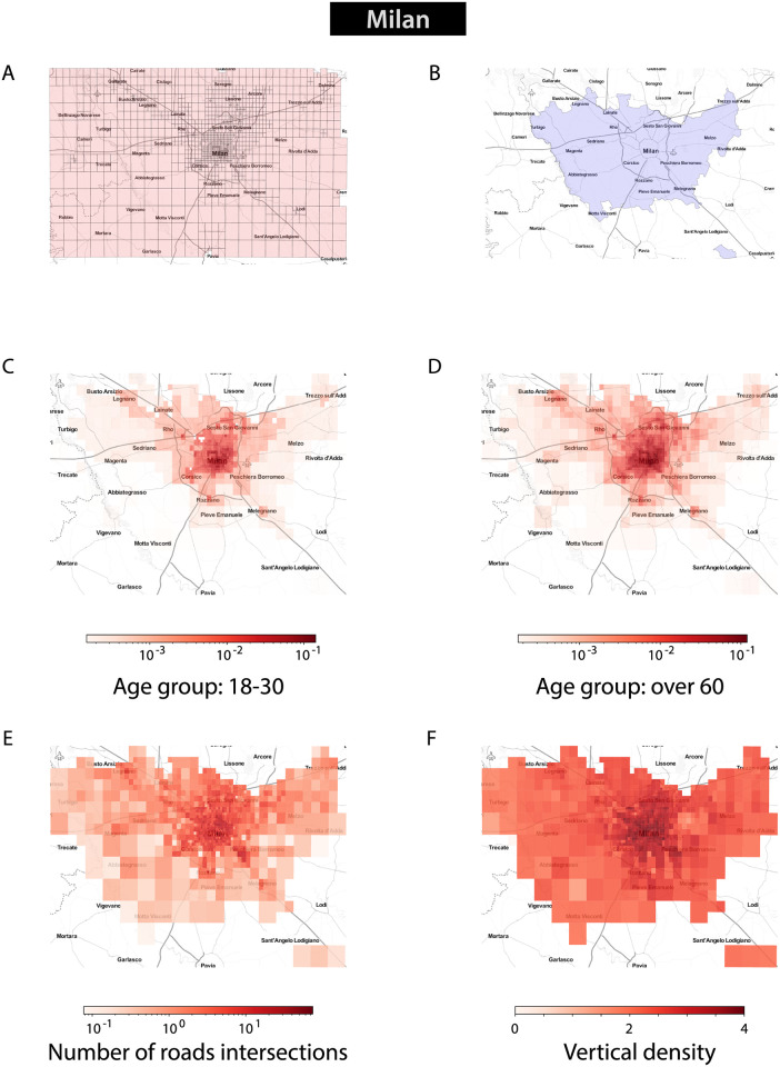
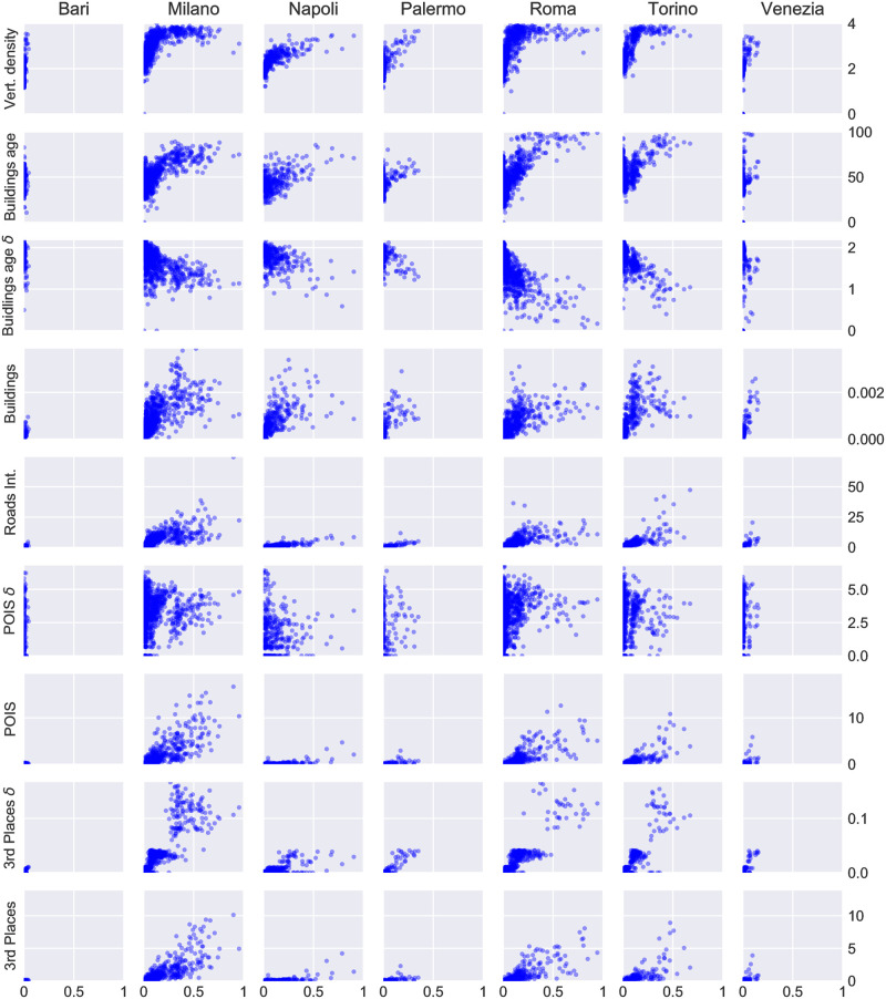
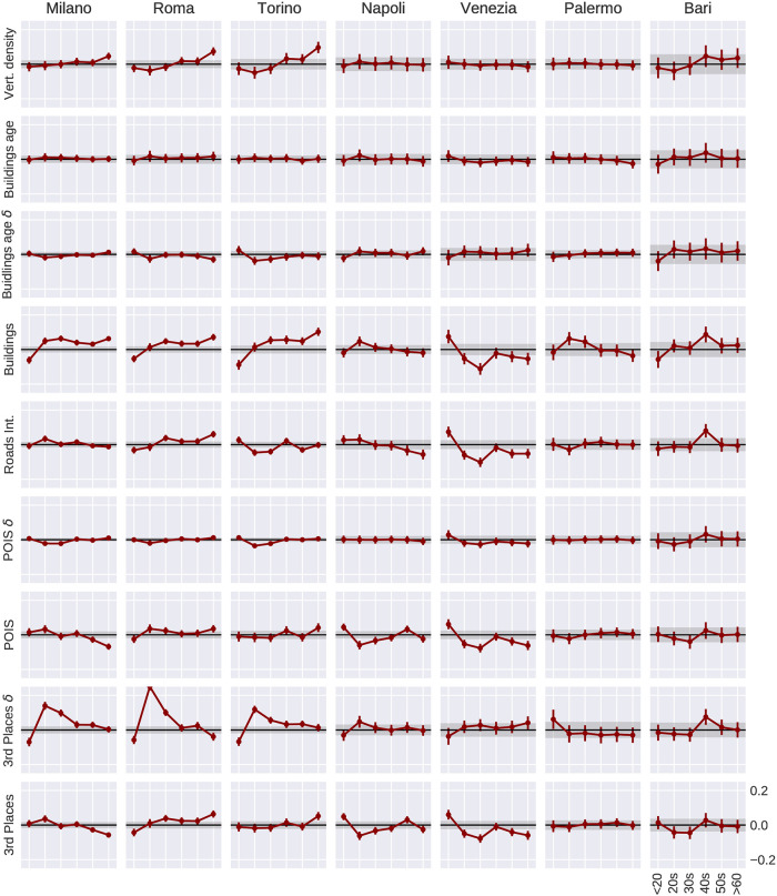
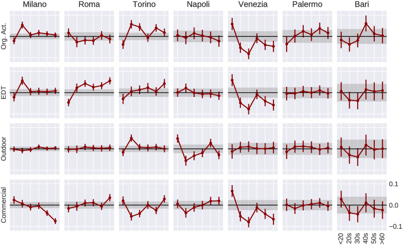
The concept of urban vibrancy has become increasingly important in the study of cities. A vibrant urban environment is an area of a city with high levels of human activity and interactions. Traditionally, studying our cities and what makes them vibrant has been very difficult, due to challenges in data collection on urban environments and people's location and interactions. Here, we rely on novel sources of data to investigate how different features of our cities may relate to urban vibrancy. In particular, we explore whether there are any differences in which urban features make an environment vibrant for different age groups. We perform this quantitative analysis by extracting urban features from OpenStreetMap and the Italian census, and using them in spatial models to describe urban vibrancy. Our analysis shows a strong relationship between urban features and urban vibrancy, and particularly highlights the importance of third places, which are urban places offering opportunities for social interactions. Our findings provide evidence that a combination of mobile phone data with crowdsourced urban features can be used to better understand urban vibrancy.
Conflict of interest statement
The authors have declared that no competing interests exist.
Figures
Similar articles
-
Effects of Urban Vibrancy on an Urban Eco-Environment: Case Study on Wuhan City.Int J Environ Res Public Health. 2022 Mar 9;19(6):3200. doi: 10.3390/ijerph19063200. Int J Environ Res Public Health. 2022. PMID: 35328888 Free PMC article.
-
The Relationship between Urban Vibrancy and Built Environment: An Empirical Study from an Emerging City in an Arid Region.Int J Environ Res Public Health. 2021 Jan 10;18(2):525. doi: 10.3390/ijerph18020525. Int J Environ Res Public Health. 2021. PMID: 33435212 Free PMC article.
-
Measuring Urban Vibrancy of Residential Communities Using Big Crowdsourced Geotagged Data.Front Big Data. 2021 Jun 10;4:690970. doi: 10.3389/fdata.2021.690970. eCollection 2021. Front Big Data. 2021. PMID: 34179770 Free PMC article.
-
The effectiveness of conservation interventions to overcome the urban-environmental paradox.Ann N Y Acad Sci. 2015 Oct;1355:1-14. doi: 10.1111/nyas.12752. Epub 2015 Apr 6. Ann N Y Acad Sci. 2015. PMID: 25845289 Review.
-
The French eco-neighbourhood evaluation model: Contributions to sustainable city making and to the evolution of urban practices.J Environ Manage. 2016 Jul 1;176:69-78. doi: 10.1016/j.jenvman.2016.03.036. Epub 2016 Mar 31. J Environ Manage. 2016. PMID: 27039366 Review.
Cited by
-
How Did the Built Environment Affect Urban Vibrancy? A Big Data Approach to Post-Disaster Revitalization Assessment.Int J Environ Res Public Health. 2022 Sep 26;19(19):12178. doi: 10.3390/ijerph191912178. Int J Environ Res Public Health. 2022. PMID: 36231479 Free PMC article.
-
Population estimation beyond counts-Inferring demographic characteristics.PLoS One. 2022 Apr 5;17(4):e0266484. doi: 10.1371/journal.pone.0266484. eCollection 2022. PLoS One. 2022. PMID: 35381028 Free PMC article.
-
Recent advances in urban system science: Models and data.PLoS One. 2022 Aug 17;17(8):e0272863. doi: 10.1371/journal.pone.0272863. eCollection 2022. PLoS One. 2022. PMID: 35976953 Free PMC article.
-
Rapid indicators of deprivation using grocery shopping data.R Soc Open Sci. 2021 Dec 22;8(12):211069. doi: 10.1098/rsos.211069. eCollection 2021 Dec. R Soc Open Sci. 2021. PMID: 34950487 Free PMC article.
-
Do Vibrant Places Promote Active Living? Analyzing Local Vibrancy, Running Activity, and Real Estate Prices in Beijing.Int J Environ Res Public Health. 2022 Dec 7;19(24):16382. doi: 10.3390/ijerph192416382. Int J Environ Res Public Health. 2022. PMID: 36554263 Free PMC article.
References
-
- DESA U. World Urbanization Prospects: 2018. New York: United Nations. 2014;.
-
- Glaeser E. Triumph of the City: How Our Greatest Invention Makes Us Richer, Smarter, Greener, Healthier, and Happier, 2011; 2011.
-
- Musterd S, Ostendorf W. Urban segregation and the welfare state: Inequality and exclusion in western cities. Routledge; 2013.
-
- Glaeser EL, Resseger M, Tobio K. Inequality in cities. Journal of Regional Science. 2009;49(4):617–646. 10.1111/j.1467-9787.2009.00627.x - DOI
MeSH terms
LinkOut - more resources
Full Text Sources
