Two-dimensional adaptive dynamics of evolutionary public goods games: finite-size effects on fixation probability and branching time

Abstract

Public goods games (PGGs) describe situations in which individuals contribute to a good at a private cost, but others can free-ride by receiving a share of the public benefit at no cost. The game occurs within local neighbourhoods, which are subsets of the whole population. Free-riding and maximal production are two extremes of a continuous spectrum of traits. We study the adaptive dynamics of production and neighbourhood size. We allow the public good production and the neighbourhood size to coevolve and observe evolutionary branching. We explain how an initially monomorphic population undergoes evolutionary branching in two dimensions to become a dimorphic population characterized by extremes of the spectrum of trait values. We find that population size plays a crucial role in determining the final state of the population. Small populations may not branch or may be subject to extinction of a subpopulation after branching. In small populations, stochastic effects become important and we calculate the probability of subpopulation extinction. Our work elucidates the evolutionary origins of heterogeneity in local PGGs among individuals of two traits (production and neighbourhood size), and the effects of stochasticity in two-dimensional trait space, where novel effects emerge.

Keywords: adaptive dynamics; ecology and evolution; evolutionary game theory.

Figure 1.

Macroscopic dynamics overview. (a) A schematic view of an initially monomorphic population branching into two distinct subpopulations, with colour indicating trait. Trait distributions are also shown for both the monomorphic and branched populations. (b) An example of the stochastic branching process, showing production over time for simulations with a population size of 1000. Each point represents an individual with its y value denoting its production and its x value denoting the generation. Six simulations with identical initial conditions are shown, with colour differentiating simulations. As predicted by deterministic theory, all of the simulations branch into two groups, one with high production and one with low production. The generation at which a simulation has branched is indicated by the arrow of the corresponding colour. The method for determining when branching occurs is detailed in §2.2. Time to branching varies even for this relatively large population size of 1000, highlighting the importance of stochasticity in our game. This stochasticity will be the focus of the following analysis, as shown in greater depth in figures 2–4. These simulations all use default parameters: β = 5, σ = 2, κ = 0.5, ω = 2 (table 1).

Figure 2.

Adaptive dynamics branching prediction. The green dot represents the producer subpopulation at the given generation in a simulation of 150 individuals, while the black dot indicates the defector subpopulation. A population size of 150 was chosen because it branches consistently, but also occasionally observes extinction events following branching. Filled contour region indicates where the defectors can exist in the deterministic limit, with the colour indicating their equilibrium frequency, p*. Blank region indicates where heterogeneity cannot exist, because either defectors (p* > 1) or producers (p* < 0) are expected to dominate based on the equilibrium frequency (see electronic supplementary material, appendix E). Arrows indicate the vector field, with opacity denoting magnitude. The solid and dashed black line indicates the equilibrium points at which the selection gradient is zero for a monomorphic population. Solid represents the attracting set, and dashed represents the repulsive set. The initial traits of the population are normally distributed with production of 0.5 and neighbourhood size of 30. ‘Default’ parameters (β = 5, σ = 2, κ = 0.5, ω = 2) were used for this simulation. (a) Immediately following initial separation, we see the subpopulations driven further apart. There is a large span in the equilibrium frequency of the subpopulations. (b) Defector subpopulation has moved little within the weak field, but producers make their way quickly towards full production and minimum neighbourhood size. The equilibrium frequency of defectors begins to settle. (c) Producers continue moving towards full production and have roughly reached minimum neighbourhood size. (d) If we let many generations pass, we see that the defector subpopulation responds to the underlying deterministic gradient, and slowly increases its neighbourhood size accordingly and settles at low production.

Figure 3.

Long-term outcomes with the same population size. Each dot represents an individual. The upper panels show a trait space view, with colour indicating generation, and dark green showing the individuals of the final generation. The solid and dashed black lines show the equilibrium points at which the selection gradient is zero for a monomorphic population. Solid represents the attracting set, and dashed represents the repulsive set. The lower panels (b,d,f) show the corresponding production trait evolution over time. Initial states of all populations are normally distributed with production of 0.5 and neighbourhood size of 30. ‘Default’ parameters (β = 5, σ = 2, κ = 0.5, ω = 2) were used for all simulations, and all simulations contain 200 individuals run for 5 million generations. A population size of 200 was chosen because it was the largest population to observe all three events (branching, no branching, and extinction). (a,b) Branching occurs, and is maintained, as noted by the two separate groups of dark green at the final generation. Red ‘X’ in b denotes branching point. The final result is a heterogeneous population. (c,d) Branching occurs, but extinction of the defector subpopulation occurs before the final generation, as noted by the lack of a dark green group in the upper left. Again, red ‘X’ in d denotes branching point. Additionally, blue ‘X’ denotes extinction point. The final result is a monomorphic population of producers, which cannot branch again. (e,f) Branching never occurs, and will never occur. The population moves out of the region where branching is possible. The result is also an all-producer population.

Figure 4.

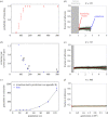
Extinction and branching events strongly depend on population size, N. One hundred simulations used for (a–b) except for N = 350 and N = 500, where only 60 were used. (a) Branching probabilities for various population sizes. The calculation of 95% confidence interval via the Agresti–Coull interval method [61]. (b) Extinction rate for various population sizes, given in the expected number of extinction events occurring in one million generations. Extinction in this case requires branching to occur first. Black circles denote example populations shown in d–f. (c) Extinction time if traits cannot mutate. In this case, we set two initial populations at minimum and maximum allowed traits (full producers and defectors), with no mutations. Note that this is a distinctly restricted model and the times to extinction are much shorter than observed in simulations with mutation, such as those shown in the other panels. Extinction occurred even if branching would not have happened first. The transition matrix approach is discussed in §3.5 and detailed further in electronic supplementary material, appendix D. Error bars for data represent the standard deviation of the mean. 300 simulations used for N = 10 − 80. One hundred simulations for N = 100 and N = 125. (d–f) Frequency of defectors for one simulation at N = 125, 175, 500, respectively. Grey shaded area indicates generations where the population was still monomorphic (e.g. before branching has occurred). Branching begins at red ‘X’. Red line indicates equilibrium frequency (p*) based on traits (see electronic supplementary material, appendix E). Green indicates plus and minus one standard deviation based on simulated data. Extinction occurs at blue ‘X’ only for d.

References

1. Rood JP. 1975. Population dynamics and food habits of the banded mongoose. Afr. J. Ecol. 13, 89–111. (10.1111/j.1365-2028.1975.tb00125.x) - DOI
1. Zomorrodi AR, Segrè D. 2017. Genome-driven evolutionary game theory helps understand the rise of metabolic interdependencies in microbial communities. Nat. Commun. 8, 1563. (10.1038/s41467-017-01407-5) - DOI - PMC - PubMed
1. Frank SA. 1998. Foundations of social evolution. Princeton, NJ: Princeton University Press.
1. Archetti M, Ferraro DA, Christofori G. 2015. Heterogeneity for IGF-II production maintained by public goods dynamics in neuroendocrine pancreatic cancer. Proc. Natl Acad. Sci. USA 112, 1833–1838. (10.1073/pnas.1414653112) - DOI - PMC - PubMed
1. Fitzpatrick BM, Fordyce JA, Gavrilets S. 2008. What, if anything, is sympatric speciation? J. Evol. Biol. 21, 1452–1459. (10.1111/j.1420-9101.2008.01611.x) - DOI - PubMed
LinkOut - more resources