Landmark-free, parametric hypothesis tests regarding two-dimensional contour shapes using coherent point drift registration and statistical parametric mapping

Abstract

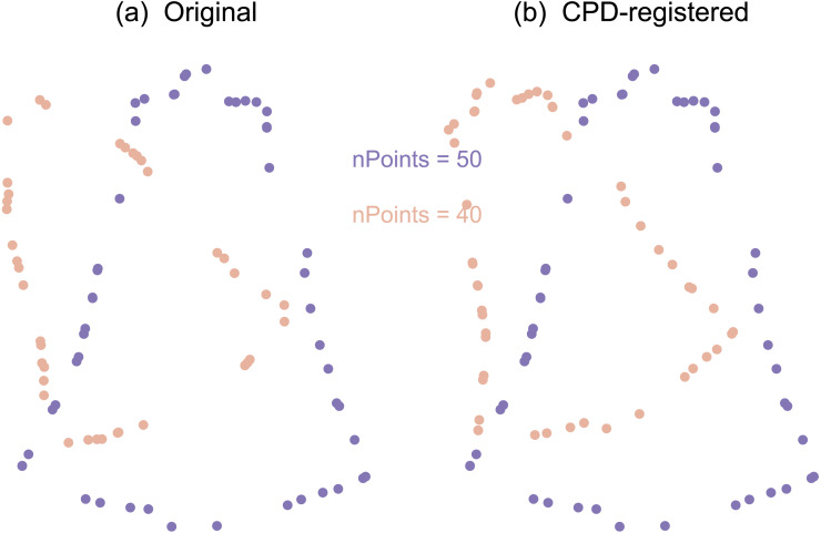
This paper proposes a computational framework for automated, landmark-free hypothesis testing of 2D contour shapes (i.e., shape outlines), and implements one realization of that framework. The proposed framework consists of point set registration, point correspondence determination, and parametric full-shape hypothesis testing. The results are calculated quickly (<2 s), yield morphologically rich detail in an easy-to-understand visualization, and are complimented by parametrically (or nonparametrically) calculated probability values. These probability values represent the likelihood that, in the absence of a true shape effect, smooth, random Gaussian shape changes would yield an effect as large as the observed one. This proposed framework nevertheless possesses a number of limitations, including sensitivity to algorithm parameters. As a number of algorithms and algorithm parameters could be substituted at each stage in the proposed data processing chain, sensitivity analysis would be necessary for robust statistical conclusions. In this paper, the proposed technique is applied to nine public datasets using a two-sample design, and an ANCOVA design is then applied to a synthetic dataset to demonstrate how the proposed method generalizes to the family of classical hypothesis tests. Extension to the analysis of 3D shapes is discussed.

Keywords: 2D shape analysis; Classical hypothesis testing; Morphology; Morphometrics; Spatial registration; Statistical analysis.

Figure 1. Overview of 2D contour data processing approaches employed in this paper.

(A) The most common analysis approach, consisting of Generalized Procrustes Analysis (GPA) and Procrustes ANOVA for landmarks. (B) Same as (A), but using mass-multivariate (MV) analysis instead of Procrustes ANOVA’s univariate (UV) approach. (C) and (D) are conceptually equivalent to (A) and (B), respectively, but operate on full contour data instead of landmark data, and can also be fully algorithmic. Statistical Parametric Mapping (SPM) is a methodology for mass-MV analysis of continuous data. See text for more details.

Figure 2. Overview of analyzed datasets.

All contour data are available in the 2D Shape Structure Dataset (Carlier et al., 2016). (A–I) For each dataset in this figure, one representative shape is highlighted, along with its numbered landmarks. Note that shape variance ranges from relatively small (e.g., Bell, Face) to relatively large (e.g., Device8, Heart).

Figure 3. Shape class exclusion examples.

Shape classes were excluded if they contained shapes with qualitatively different contour geometry. For example: (A) the ‘cup’ class was excluded because some shapes had unattached handles with holes and others had attached handles without holes. (B) The ‘octopus’ class was excluded because the eight appendages appeared in non-homologous locations.

Figure 4. Example point set registration using the coherent point drift (CPD) algorithm.

(A) Original. (B) CPD-registered. Note that CPD requires neither corresponding points, nor an equal number of points.

Figure 5. Example optimum roll correspondence.

(A) Original data, consisting of an equal number of contour points, arranged in a random order. (B) Ordered points; clockwise along the contour. (C) Rolled points; moving the initial point of contour B brings the shapes into better correspondence. (D) Optimally rolled points; the total deformation energy across all points (i.e., the sum-of-squared correspondence line lengths) is minimum.

Figure 6. Example parametric representations of 2D contour shape.

Dots represent manually defined landmarks, and are shown as visual references. Left panel (XY plane): the spatial plane in which shape data are conventionally presented. The three colors represent different shapes. Bottom panel (UX plane) and right panel (UY plane): abstract planes in which U represents the parametric position (from 0 to 1) along the contour; positions U = 0 and U = 1 are equivalent.

Figure 7. Landmark results from mass-multivariate testing.

(A–I) Landmark-specific T² values are presented along with the critical threshold at α = 0.05, and probability values for the overall mass-multivariate test.

Figure 8. Contours mass-multivariate results using Statistical Parametric Mapping (SPM).

(A–I) Results for both parametric and nonparametric inference are shown. P values represent the probability that random variation in the Mean A contour would produce a deformation as large as in the observed Mean B, given the estimated contour variance. Dots on the Mean B contour represent contour points whose T² values exceeded the threshold for significance at α = 0.05; if the maximum T² value did not reach this threshold, the p value is greater than α, and no dots are shown.

Figure 9. Example MANCOVA using synthetic data; for simplicity, data were generated to have (i) a relatively large signal:noise ratio, and (ii) close-to-perfect correspondence, by sampling at 101 equally spaced angular distances around the contour.

(A) The original contour dataset, consisting of five noisy circles for each of two groups, with systematically different mean radii, and also with both group- and size-dependent signal, where ‘size’ was considered to be the mean radius, and where ‘signal’ implies true morphological difference. Note that the size-dependent signal is more easily perceived in (A), and that the group-dependent signal is more easily perceived in the next panel. (B) Registered contours. (C, D) Size effects from MANCOVA for the original and registered data; the test statistic is presented as $\sqrt{T^2}$ because a linear T² scale would result in imperceivable color differences (i.e., the (C) points would be all white, and the points in the other panels would all be close-to-black). (E, F) Group effects from MANCOVA for the original and registered data; note that the (E) and (F) results are similar because MANCOVA accounts for size-related effects in the ‘Original’ data.

Figure 10. Example 3D surface unwrapping.

(A) Original 3D geometry. (B) Unwrapped geometry; this is a 2D parametric (UV) representation of the original geometry. Colors represent changes in surface normal direction. The thick black line in (A) represents a seam along which the 3D geometry is cut so that it can be flattened into a 2D shape. Unwrapping was performed here using boundary first flattening (Sawhney & Crane, 2017).

Figure 11. Example processing sensitivity.

Case 1 (A–B) depicts the result reported in Fig. 8G. Case 2 (C–D) depicts the results after point re-shuffling (i.e., a new random points order, see Fig. 5A), then re-application of the processing chain depicted in Fig. 1D. Note: results for Case 1 were qualitatively replicated for most random re-shufflings, but approximately 1 in 20 re-shufflings yielded qualitatively different results, like those depicted for Case 2.

References

1. Adams DC, Otárola-Castillo E. Geomorph: an R package for the collection and analysis of geometric morphometric shape data. Methods in Ecology and Evolution. 2013;4(4):393–399. doi: 10.1111/2041-210X.12035. - DOI
1. Adams DC, Rohlf FJ, Slice DE. Geometric morphometrics: ten years of progress following the ‘revolution’. Italian Journal of Zoology. 2004;71(1):5–16. doi: 10.1080/11250000409356545. - DOI
1. Adams DC, Rohlf FJ, Slice DE. A field comes of age: geometric morphometrics in the 21st century. Hystrix. 2013;24(1):7.
1. Adler RJ, Taylor JE. Random fields and geometry. Springer-Verlag; New York: 2007.
1. Anaconda Anaconda software distribution version 3-6.10. 2020. https://anaconda.com https://anaconda.com