. 2021:52:587-601.
doi: 10.1016/j.arcontrol.2021.05.001. Epub 2021 May 28.

Dynamical characterization of antiviral effects in COVID-19

Affiliations

Dynamical characterization of antiviral effects in COVID-19

Pablo Abuin et al. Annu Rev Control. 2021.

Abstract

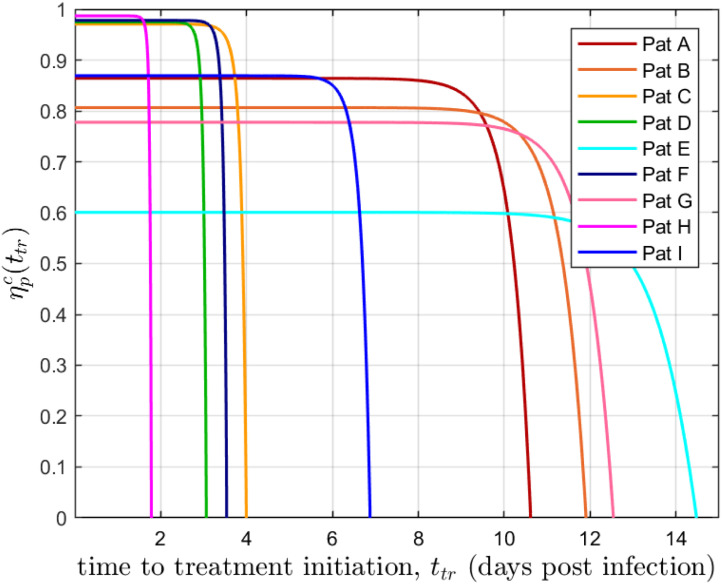
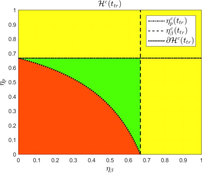
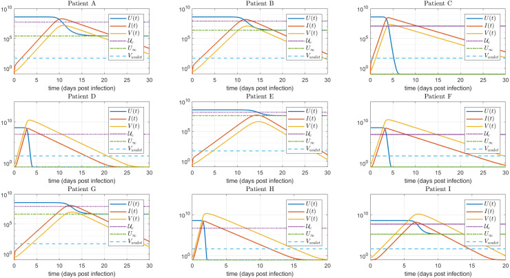
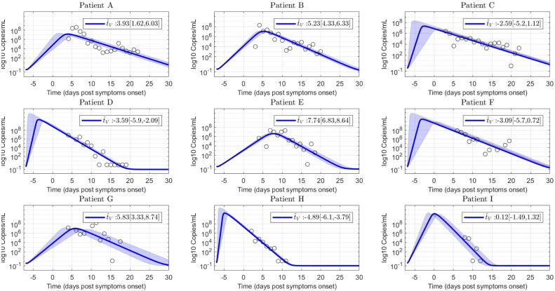
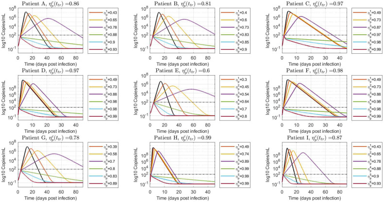
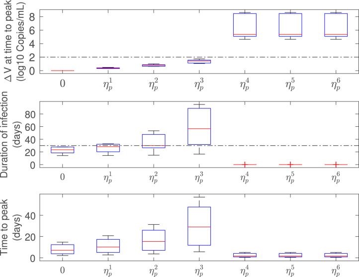
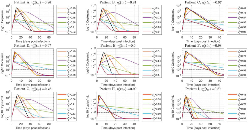
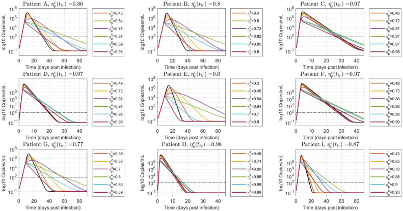
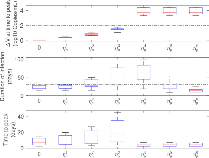
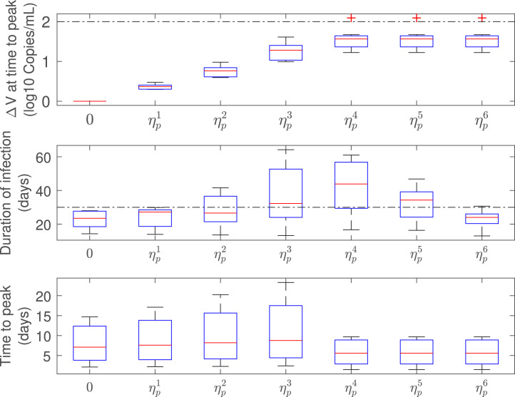
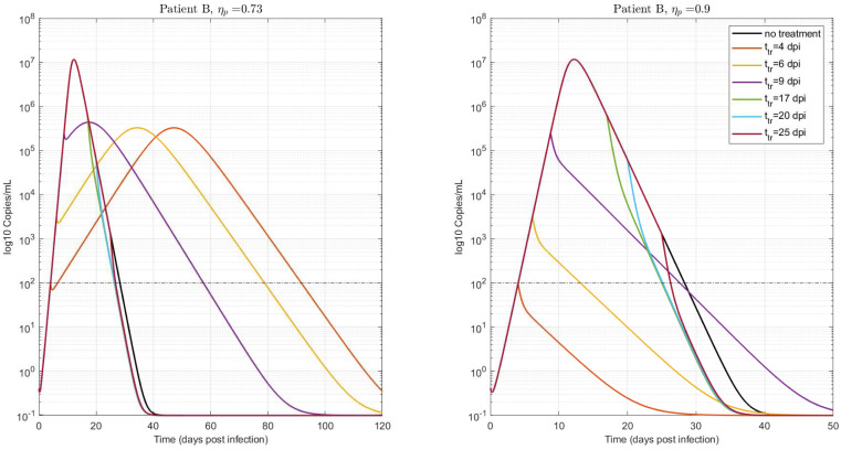
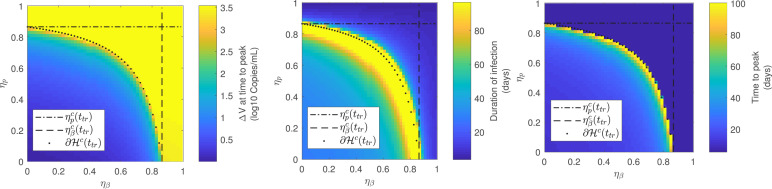
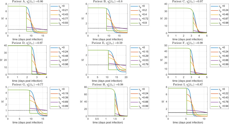
Mathematical models describing SARS-CoV-2 dynamics and the corresponding immune responses in patients with COVID-19 can be critical to evaluate possible clinical outcomes of antiviral treatments. In this work, based on the concept of virus spreadability in the host, antiviral effectiveness thresholds are determined to establish whether or not a treatment will be able to clear the infection. In addition, the virus dynamic in the host - including the time-to-peak and the final monotonically decreasing behavior - is characterized as a function of the time to treatment initiation. Simulation results, based on nine patient data, show the potential clinical benefits of a treatment classification according to patient critical parameters. This study is aimed at paving the way for the different antivirals being developed to tackle SARS-CoV-2.

Keywords: Antiviral effectiveness; Dynamic characterization; In-host model; SARS-CoV-2.


Conflict of interest statement

The authors declare that they have no known competing financial interests or personal relationships that could have appeared to influence the work reported in this paper.

Figures

Fig. 1
Fig. 1
ηpc(ttr) vs ttr corresponding to the nine patients simulated in Section 4. . The nine COVID-19 patients (A, B, C, D, E, F, G, H and I) identified from data sets in (Wölfel et al. (2020)) are represented here as ”pat”.
Fig. 2
Fig. 2
Hc(ttr) is given by the yellow and the green regions, considering the following system parameters: β=0.5, δ=0.2, p=2 and c=5, with U(ttr)=3. The critical boundary of Hc(ttr), denoted by Hc(ttr), represents the critical pairs of ηβ and ηp such that R(ttr)=1. (For interpretation of the references to color in this figure legend, the reader is referred to the web version of this article.)
Fig. 3
Fig. 3
U, I, V time evolution for the untreated case. As stated in Theorem 4.1, in Abuin et al. (2020), tˇV<tˆI<tc<tˆV, where tˇV and tˆV are the times at which V(t) reaches a local minimum and a local maximum, respectively, tˆI is the time at which I(t) reaches a local maximum, and tc is the time at which U(t) reaches Uc. Furthermore, as stated in Appendix A.2, tˇV0 and tˆItctˆV. Vundet=100 (copies/mL) stands for the undetectable level of the virus load.
Fig. 4
Fig. 4
Uncertainty analysis on viral load evolution for p-parameter 95% confidence interval. Note the uncertainty in viral load peak. Empty dots are data of COVID-19 patients.
Fig. 5
Fig. 5
Free virus behavior when treatment is started at viral load detection level (ttr=tDL). Values of ηp smaller (ηp1,ηp2), approximately equal (ηp3,ηp4) and greater (ηp5,ηp6) than ηpc are simulated to demonstrate the results in Theorem 3.1. The black line denotes the untreated case (ηp=0).
Fig. 6
Fig. 6
Infection-related metrics as function of ηp (ttr=tDL), for antiviral effectiveness assessment (all patients). Note that, ηp1=0.5ηpc(ttr), ηp2=0.75ηpc(ttr), ηp3=0.90ηpc(ttr), ηp4=ηpc(ttr)+0.1(1ηpc(ttr)), ηp5=ηpc(ttr)+0.25(1ηpc(ttr)), and ηp6=ηpc(ttr)+0.5(1ηpc(ttr)), being ηpc(ttr) the critical drug efficacy of each patient at time to treatment initiation, ttr.
Fig. 7
Fig. 7
Viral load time evolution with treatment initial time given by ttr=0.7te. Values of ηp smaller, approximately equal and greater than ηpc are simulated to demonstrate the results in Theorem 3.1. The black line denotes the untreated case (ηp=0).
Fig. 8
Fig. 8
Viral load time evolution with treatment initial time given by ttr=te. Values of ηp smaller, approximately equal and greater than ηpc are simulated to demonstrate the results in Theorem 3.1. The black line denotes the untreated case (ηp=0).
Fig. 9
Fig. 9
Infection-related metrics as function of ηp (ttr=0.7te), for antiviral effectiveness assessment (all patients).
Fig. 10
Fig. 10
Infection-related metrics as function of ηp (ttr=te), for antiviral effectiveness assessment (all patients).
Fig. 11
Fig. 11
Virus time evolution for different treatment times, ttr=4,6,8,17,20,25 (dpi). Two fixed values of ηp were used, smaller and bigger than ηpc(ttr): ηp=0.73 (left) and ηp=0.9 (right), respectively. ηpc(ttr)0.81 for ttr<te. Patient B. .
Fig. 12
Fig. 12
Infection-related metrics for antiviral effectiveness assessment as function of ηp and ηβ (ttr=0.7te). Patient A.. (For interpretation of the references to color in this figure legend, the reader is referred to the web version of this article.)
Fig. 13
Fig. 13
Qualitative plot of function f(V) (arbitrary parameters) for different values of R. As it can be seen – independently of the parameter values – if R(ttr)>1 it there exists an interval of values of V, and a corresponding period of time such that f(V)>V.
Fig. 14
Fig. 14
Evolution of R(t) when an antiviral treatment is initiated at a time of approximately 0.75tˆV, and different antiviral inhibition effects ηp are considered, smaller and greater than the critical value ηpc. The black dashed line represents R=1. As it can be seen, for values of ηp<ηpc, R(t) crosses 1 at larger times for larger values of ηp as it is stated in Lemma 1. This implies that if ηp<ηpc, larger values of ηp delays the virus peak time, as it is stated in Theorem 3.1.iii. Furthermore, the figure confirms that, for real patient date, te is close to tˆV.
Fig. 15
Fig. 15
Phase portrait of system (2.1) with parameters β=0.5, δ=0.2, p=2 and c=5, for different initial conditions not necessarily representing realistic cases. Empty circles represent the initial state, while solid circles represent final states. The red hyperplane corresponds to U(t)Uc (i.e., the critical value of U, when R(t)=1) while the blue hyperplane corresponds to the fast manifold in which I(t) and V(t) are proportional (.i.e, I(t)=cpV(t)). Note that only the initial states with U0>Uc=1 corresponds to scenarios with R0>1.

Similar articles

Cited by

References

    1. Abuin P., Anderson A., Ferramosca A., Hernandez-Vargas E.A., Gonzalez A.H. Characterization of SARS-CoV-2 dynamics in the host. Annual Reviews in Control. 2020;50:457–468. - PMC - PubMed
    1. Baccam P., Beauchemin C., Macken C.A., Hayden F.G., Perelson A.S. Kinetics of influenza a virus infection in humans. Journal of Virology. 2006;80(15):7590–7599. - PMC - PubMed
    1. Callaway D.S., Perelson A.S. HIV-1 infection and low steady state viral loads. Bulletin of Mathematical Biology. 2002;64(1):29–64. - PubMed
    1. Cao Y., Hiyoshi A., Montgomery S. COVID-19 case-fatality rate and demographic and socioeconomic influencers: worldwide spatial regression analysis based on country-level data. BMJ Open. 2020;10(11) - PMC - PubMed
    1. Cao P., McCaw J.M. The mechanisms for within-host influenza virus control affect model-based assessment and prediction of antiviral treatment. Viruses. 2017;9(8):197. - PMC - PubMed

LinkOut - more resources