

A partition of unity approach to fluid mechanics and fluid-structure interaction
- PMID: 34093912
- PMCID: PMC7610902
- DOI: 10.1016/j.cma.2020.112842
A partition of unity approach to fluid mechanics and fluid-structure interaction
Abstract
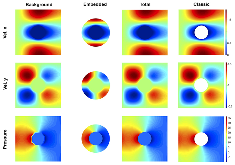
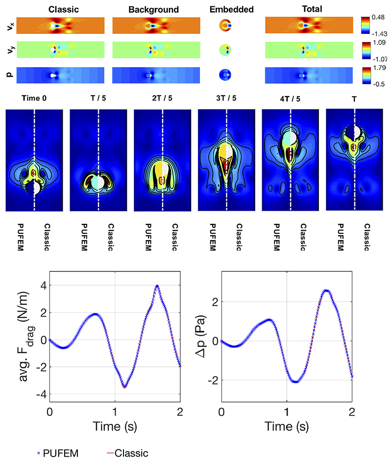
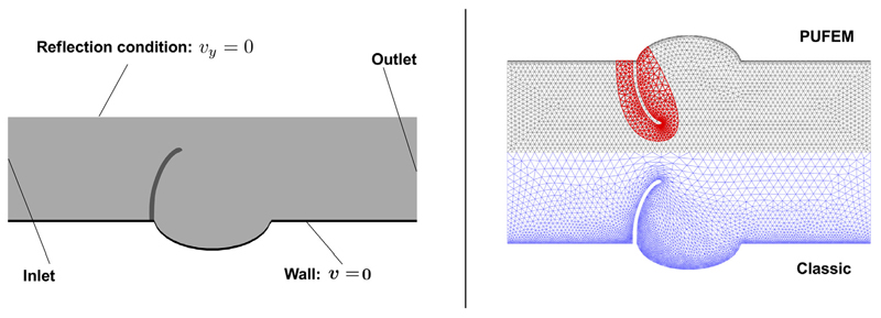
For problems involving large deformations of thin structures, simulating fluid-structure interaction (FSI) remains a computationally expensive endeavour which continues to drive interest in the development of novel approaches. Overlapping domain techniques have been introduced as a way to combine the fluid-solid mesh conformity, seen in moving-mesh methods, without the need for mesh smoothing or re-meshing, which is a core characteristic of fixed mesh approaches. In this work, we introduce a novel overlapping domain method based on a partition of unity approach. Unified function spaces are defined as a weighted sum of fields given on two overlapping meshes. The method is shown to achieve optimal convergence rates and to be stable for steady-state Stokes, Navier-Stokes, and ALE Navier-Stokes problems. Finally, we present results for FSI in the case of 2D flow past an elastic beam simulation. These initial results point to the potential applicability of the method to a wide range of FSI applications, enabling boundary layer refinement and large deformations without the need for re-meshing or user-defined stabilization.
Keywords: Finite element methods; Fluid–structure interaction; Overlapping domains; Partition of unity.
Figures


Similar articles
-
A sharp interface Lagrangian-Eulerian method for flexible-body fluid-structure interaction.J Comput Phys. 2023 Sep 1;488:112174. doi: 10.1016/j.jcp.2023.112174. Epub 2023 Apr 24. J Comput Phys. 2023. PMID: 37214277 Free PMC article.
-
Fluid-Structure Interaction Simulation of Prosthetic Aortic Valves: Comparison between Immersed Boundary and Arbitrary Lagrangian-Eulerian Techniques for the Mesh Representation.PLoS One. 2016 Apr 29;11(4):e0154517. doi: 10.1371/journal.pone.0154517. eCollection 2016. PLoS One. 2016. PMID: 27128798 Free PMC article.
-
Fluid-structure interaction involving large deformations: 3D simulations and applications to biological systems.J Comput Phys. 2014 Feb 1;258:10.1016/j.jcp.2013.10.047. doi: 10.1016/j.jcp.2013.10.047. J Comput Phys. 2014. PMID: 24415796 Free PMC article.
-
Fluid-structure interaction modeling in cardiovascular medicine - A systematic review 2017-2019.Med Eng Phys. 2020 Apr;78:1-13. doi: 10.1016/j.medengphy.2020.01.008. Epub 2020 Feb 17. Med Eng Phys. 2020. PMID: 32081559
-
A Robust Adaptive Mesh Generation Algorithm: A Solution for Simulating 2D Crack Growth Problems.Materials (Basel). 2023 Sep 29;16(19):6481. doi: 10.3390/ma16196481. Materials (Basel). 2023. PMID: 37834618 Free PMC article. Review.
Cited by
-
A class of analytic solutions for verification and convergence analysis of linear and nonlinear fluid-structure interaction algorithms.Comput Methods Appl Mech Eng. 2020 Apr 15;362:112841. doi: 10.1016/j.cma.2020.112841. eCollection 2020 Apr 15. Comput Methods Appl Mech Eng. 2020. PMID: 34093913 Free PMC article.
-
Ascitic Shear Stress Activates GPCRs and Downregulates Mucin 15 to Promote OvarianCancer Malignancy.Res Sq [Preprint]. 2024 Nov 25:rs.3.rs-5160301. doi: 10.21203/rs.3.rs-5160301/v2. Res Sq. 2024. PMID: 39483899 Free PMC article. Preprint.
References
-
- Stein K, Benney R, Kalro V, Johnson A, Tezduyar T, Stein K, Benney R, Kalro V, Johnson A, Tezduyar T. Parallel computation of parachute fluid-structure interactions; 14th Aerodynamic Decelerator Systems Technology Conference; 1997. p. 1505.
-
- Kalro V, Tezduyar TE. A parallel 3D computational method for fluid–structure interactions in parachute systems. Comput Methods Appl Mech Engrg. 2000;190(3-4):321–332.
-
- Takizawa K, Spielman T, Tezduyar TE. Space-time FSI modeling and dynamical analysis of spacecraft parachutes and parachute clusters. Comput Mech. 2011;48(3):345.
-
- Bazilevs Y, Hsu M-C, Akkerman I, Wright S, Takizawa K, Henicke B, Spielman T, Tezduyar T. 3D simulation of wind turbine rotors at full scale. Part I: geometry modelling and aerodynamics. InterNat J Numer Methods Fluids. 2011;65(1-3):207–235.
-
- Bazilevs Y, Hsu M-C, Kiendl J, Wüchner R, Bletzinger K-U. 3D simulation of wind turbine rotors at full scale. Part II: fluid-structure interaction modelling with composite blades. Inter Nat J Numer Methods Fluids. 2011;65(1-3):236–253.
Grants and funding
LinkOut - more resources
Full Text Sources
Miscellaneous