Learning divisive normalization in primary visual cortex

Abstract

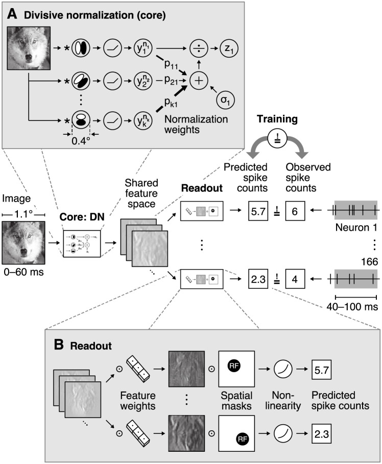
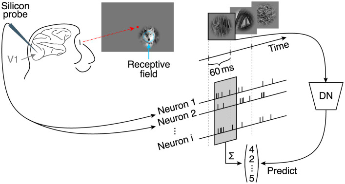
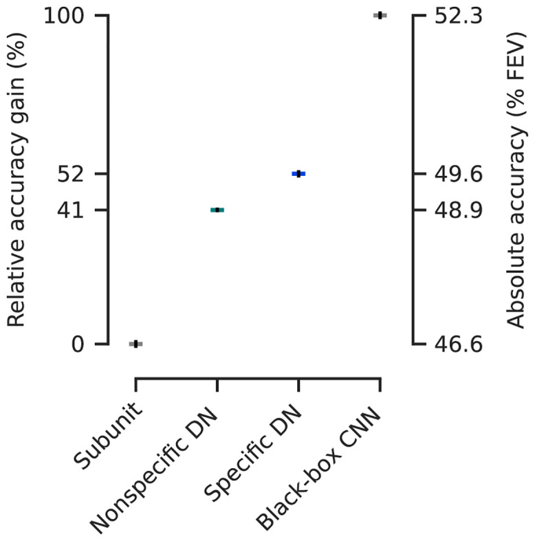
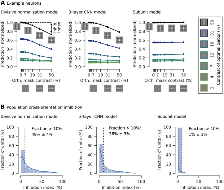
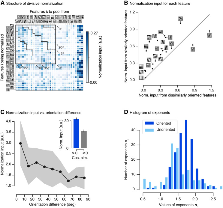
Divisive normalization (DN) is a prominent computational building block in the brain that has been proposed as a canonical cortical operation. Numerous experimental studies have verified its importance for capturing nonlinear neural response properties to simple, artificial stimuli, and computational studies suggest that DN is also an important component for processing natural stimuli. However, we lack quantitative models of DN that are directly informed by measurements of spiking responses in the brain and applicable to arbitrary stimuli. Here, we propose a DN model that is applicable to arbitrary input images. We test its ability to predict how neurons in macaque primary visual cortex (V1) respond to natural images, with a focus on nonlinear response properties within the classical receptive field. Our model consists of one layer of subunits followed by learned orientation-specific DN. It outperforms linear-nonlinear and wavelet-based feature representations and makes a significant step towards the performance of state-of-the-art convolutional neural network (CNN) models. Unlike deep CNNs, our compact DN model offers a direct interpretation of the nature of normalization. By inspecting the learned normalization pool of our model, we gained insights into a long-standing question about the tuning properties of DN that update the current textbook description: we found that within the receptive field oriented features were normalized preferentially by features with similar orientation rather than non-specifically as currently assumed.

Fig 1. Overview of our divisive normalization (DN) model.

The model takes as input an image covering 1.1° of visual field and predicts neurons’ spike counts in response to this image (details in Fig 2). The model is split into two parts: a core that computes a shared nonlinear feature space and a readout that maps the shared feature space individually to each neuron’s spike count. A. Divisive normalization mechanism (simplified). The visual input is convolved with 32 filters covering 0.4° of visual field and then rectified and exponentiated to produce an excitatory output. The output of each filter is then divided by a weighted sum of the excitatory outputs of all filters with normalization weights p_kl and a semi-saturation constant σ_l. In our general formulation, all weights and constants are learned from the data. B. Readout that maps the shared feature space to each neuron’s spike count through an individual weighted sum over the entire shared feature space and a pointwise output nonlinearity. The readout weights are factorized into a feature vector—capturing the nonlinear feature(s) that a neuron computes—and a spatial mask—localizing each neuron’s receptive field (RF).

Fig 2. Experimental paradigm from Cadena and colleagues [14].

Natural images were flashed to a monkey covering 2° of their visual angle, and located at the center of the multi-unit receptive field. Multiple neurons were isolated from recordings with silicon probes inserted into V1 [41]. Natural images were shown in a fast sequence without blanks, each presented for 60 ms. Spike counts from all isolated neurons corresponding to each image were extracted from a window 40 ms after the image onset lasting 60 ms.

Fig 3. Performance comparison of our models fitted to the data from Cadena and colleagues [14] relative to the gap between the best shallow model—a subunit one layer convolutional neural network (CNN)—and the deeper data-driven state-of-the-art three-layer CNN [14].

Non-specific divisive normalization (DN) accounts for 41% of this gap, while specific DN improves it up to 52%. Absolute values in terms of percentage of explainable variance explained (FEV) on the right (mean over the ten best models selected in terms of validation set accuracy, see main text for details). Error-bars (black) indicate the standard error of the mean. Model performance is significantly different between each model class (pairwise Wilcoxon signed rank test on best models in terms of validation accuracy: p < 0.024, N = 166 neurons, family-wise error rate α = 0.05 using Holm-Bonferroni correction).

Fig 4. Cross-orientation inhibition was learned by our DN model and the three-layer CNN, but not significantly by the subunit model.

A. Tuning curves for an example neuron of all three models and various contrast combinations of the optimal Gabor (box on the right, examples for contrasts of 0%, 1% and 2% not shown) and an orthogonal Gabor masking. As the contrast of the orthogonal mask increases, the model prediction (normalized by the maximum response) decreases. The cross-orientation inhibition (inhib.) index measures the percentage of response inhibition by adding the masking compared to the optimal Gabor presented alone, in this case approximately 20%. A. insets: Illustration of plaid stimuli, created by overlaying an optimally oriented Gabor with an orthogonal mask. B. Histograms of the cross-orientation inhibition indices accumulated across the best ten models (in terms of validation set accuracy) per model type, with kernel density estimate of the underlying distribution. The fraction of cells that show more than 10% cross-orientation inhibition is displayed right of the dotted line (mean and 95% confidence interval over the ten best models selected in terms of validation set accuracy). For the DN model, more cells show cross-orientation inhibition compared to the other models. The subunit model shows almost no cross-orientation inhibition.

Fig 5. Structure of divisive normalization.

A. The matrix shows the average strength of the normalizing inputs (products ${\langle p_{kl}{y}_k^{n_k}\left(x\right)\rangle }_x$ in denominator of Eq (1) averaged across images; see Methods) for each combination of filter response being normalized (rows) and filter response providing normalizing input (columns). Darker shades of blue indicate stronger normalization. Orientation-selective filters are grouped at the top, ordered by preferred orientation and marked by the black square. The dashed black lines within the square separate pairs of filters with similar (< 45°) and dissimilar (≤ 45°) orientations. Normalizing inputs are stronger for similarly tuned filters. Unoriented filters mainly accounting for orientation-unspecific contrast are sorted by total normalization input. Darkest blue color corresponds to the maximum normalization input for the group of oriented filters, higher normalization input values for the unoriented filters are clipped to that value. Data of the model with highest accuracy on the validation set is shown. B. Normalization input from similar orientations (< 45°) compared to the normalization input from dissimilar orientations (≥ 45°) for each oriented linear filter. Grey line: identity. Most features are normalized preferentially by the responses of filters with similar preferred orientations. Data of the model with highest accuracy on the validation set is shown. C. Normalization input, binned into orientation difference of 10°. Each bin was averaged over the top-10 models (assessed on the validation set). The shaded area depicts the standard deviation per bin. C inset. Normalization input (norm. input) vs. cosine similarity between linear filters (cos. sim.) averaged across the top-10 models (assessed on the validation set). A cosine similarity greater than zero corresponds to similar features. Error bars: standard error of the mean. D. Histogram of DN exponents (n_l in Eq 1) of the ten best performing models in terms of validation set accuracy. Darker/lighter color: exponents corresponding to driving inputs due to oriented/unoriented linear filters. Most values are larger than one, with a few exceptions mainly corresponding to unoriented filters.

Fig 6. Histogram of feature readout weights of the ten best performing models in terms of validation set accuracy.

For each model, feature weights are normalized across channels and averaged across individual neurons. All model’s channels are used to predict neural activity.

Fig 7. Size-tuning in silico experiments and spatially extended DN control models.

A. inset: Prediction of the best DN model (chosen by validation set accuracy) for all neurons to gratings of increasing size. The gratings’ properties were determined from the units’ optimally stimulating Gabor pattern. As grating diameter increased, only very few neurons showed mostly weak suppression. Predictions normalized to maximum response per neuron. Suppression index measures asymptotic suppression relative to the maximum prediction A. main panel: Across all neurons and the ten best DN models (chosen by validation set accuracy), almost no neurons show significant surround suppression. B. Test set performance of the ten best performing DN models. The model’s performance rapidly decreases for spatially increasing normalization pool size (in units of visual angle in degrees). The best model on the validation set is indicated by a blue dot. C. & D. Weights of the spatial normalization pool for the best performing model with pool size of (C.) 1.06° of visual field (5 px × 5 px) and (D.) 1.34° of visual field (7 px × 7 px; all evaluated in terms of the validation set accuracy). For each feature (columns), the two components (rows) of the in total 32 spatial normalization pools are shown. Darker color corresponds to higher weights. Both components are similar. B. insets: Average across features and normalization pool components. The model learned normalization from the receptive field center (on average).

References

1. Carandini M, Demb JB, Mante V, Tolhurst DJ, Dan Y, Olshausen BA, et al. Do we know what the early visual system does? Journal of Neuroscience. 2005;25:10577–10597. doi: 10.1523/JNEUROSCI.3726-05.2005 - DOI - PMC - PubMed
1. Simoncelli EP, Paninski L, Pillow J, Schwartz O. Characterization of neural responses with stochastic stimuli. The Cognitive Neurosciences. 2004;3:327–338.
1. Adelson EH, Bergen JR. Spatiotemporal Energy Models for the Perception of Motion. Journal of the Optical Society of America A. 1985;2:284–299. doi: 10.1364/JOSAA.2.000284 - DOI - PubMed
1. Rust NC, Schwartz O, Movshon JA, Simoncelli EP. Spatiotemporal Elements of Macaque V1 Receptive Fields. Neuron. 2005;46:945–956. doi: 10.1016/j.neuron.2005.05.021 - DOI - PubMed
1. Touryan J, Felsen G, Dan Y. Spatial structure of complex cell receptive fields measured with natural images. Neuron. 2005;45(5):781–791. doi: 10.1016/j.neuron.2005.01.029 - DOI - PubMed
Publication types