Localization atomic force microscopy

Abstract

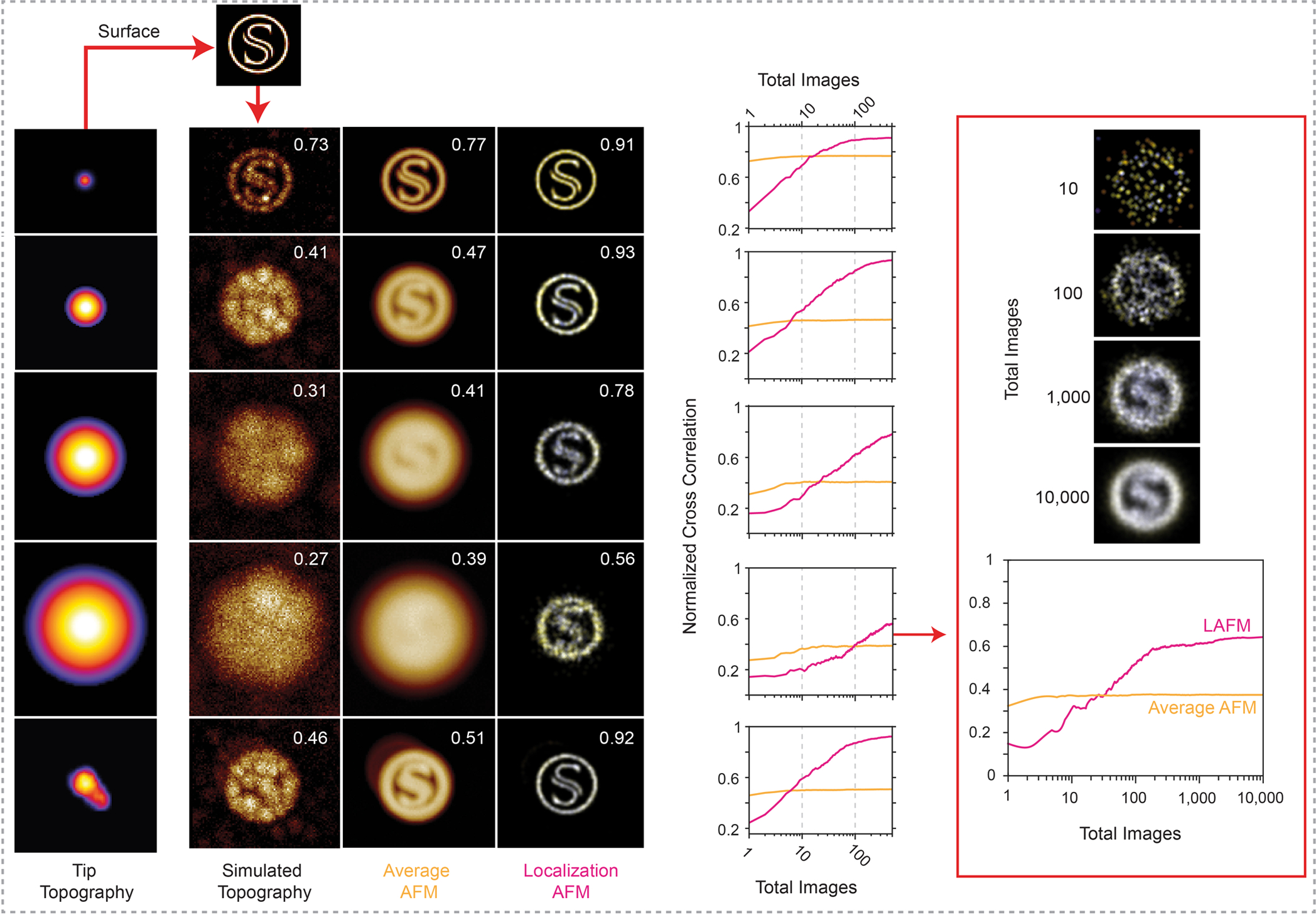
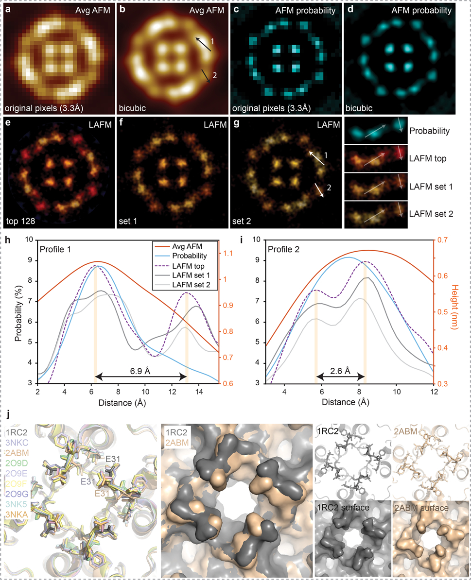
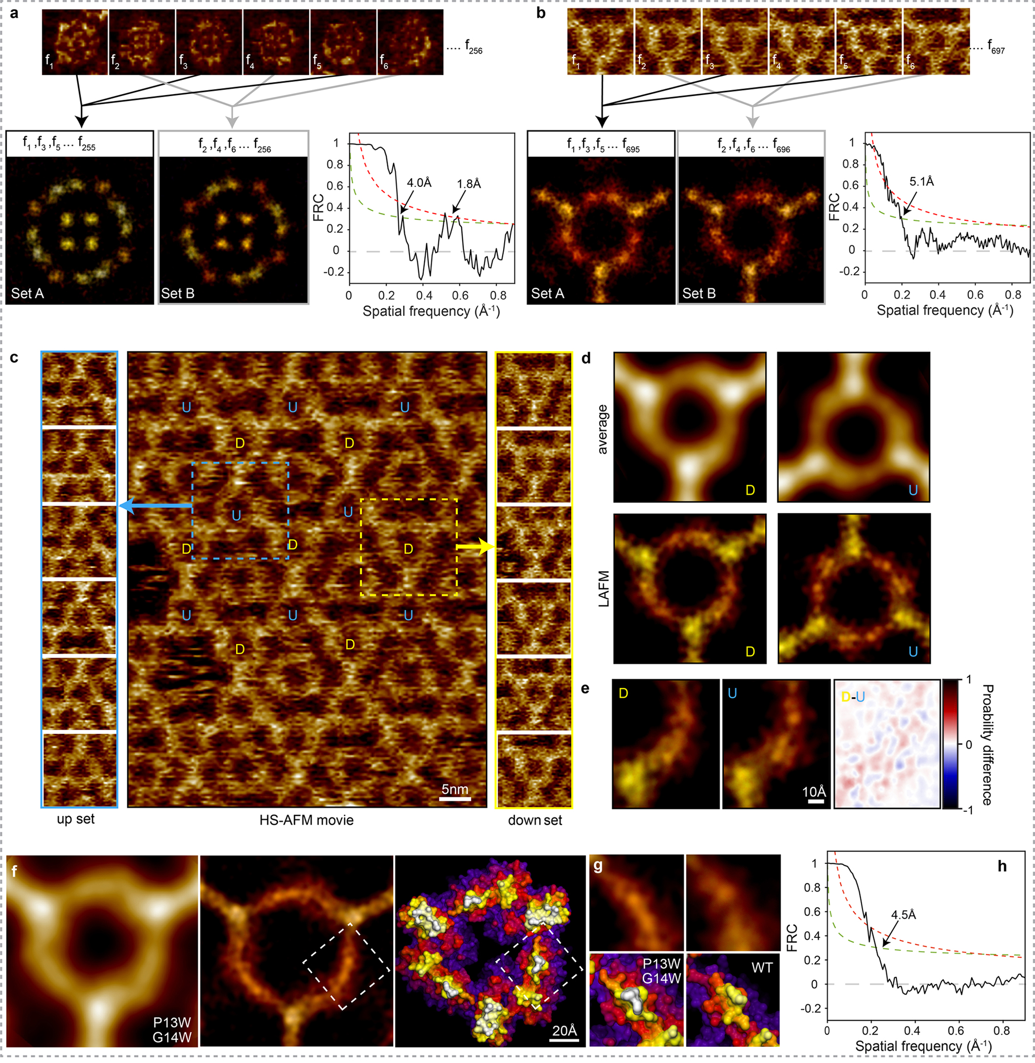
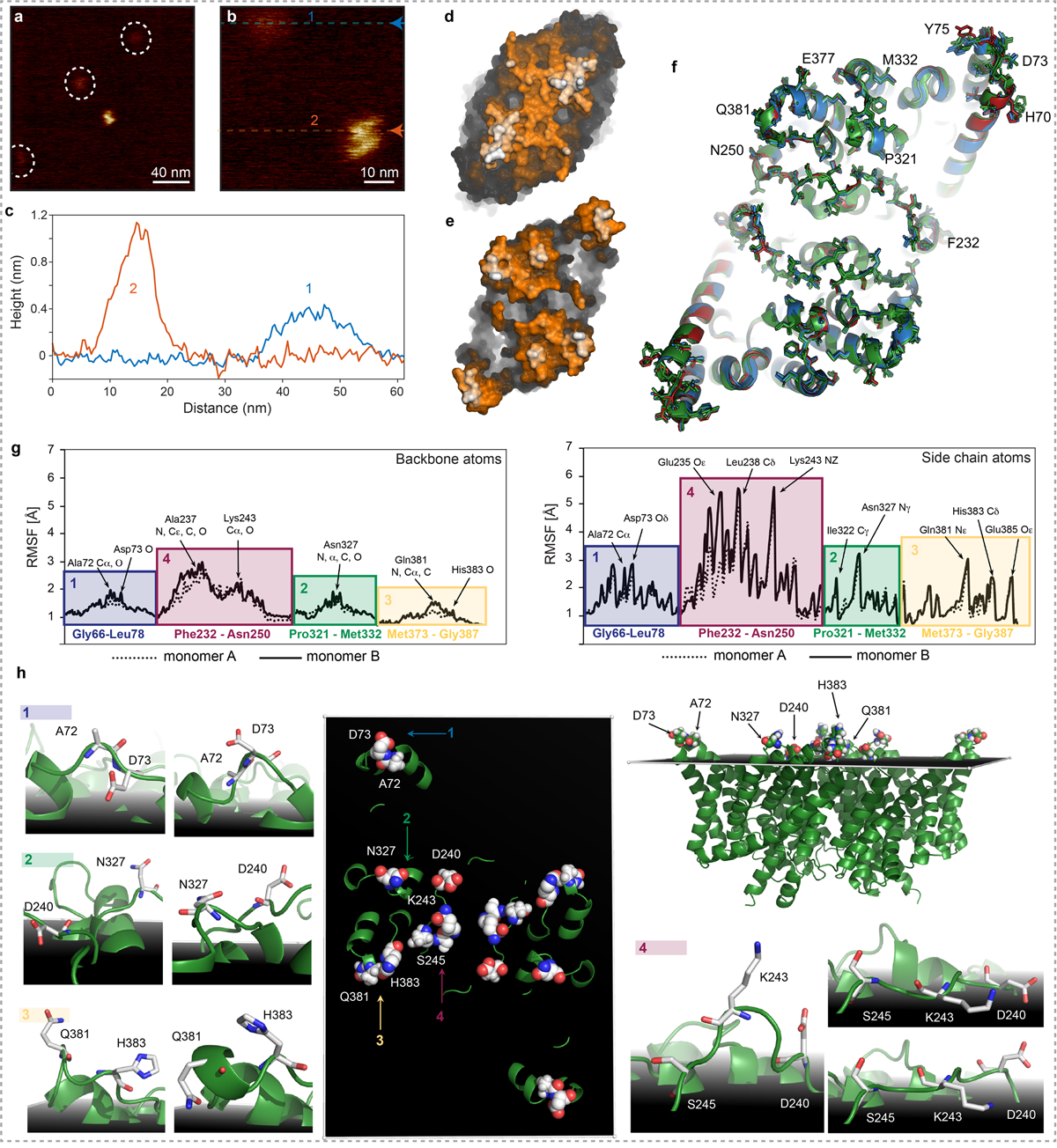
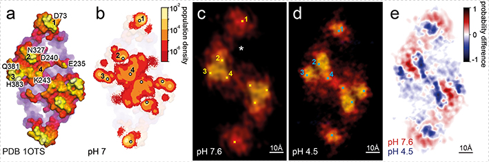
Understanding structural dynamics of biomolecules at the single-molecule level is vital to advancing our knowledge of molecular mechanisms. Currently, there are few techniques that can capture dynamics at the sub-nanometre scale and in physiologically relevant conditions. Atomic force microscopy (AFM)¹ has the advantage of analysing unlabelled single molecules in physiological buffer and at ambient temperature and pressure, but its resolution limits the assessment of conformational details of biomolecules². Here we present localization AFM (LAFM), a technique developed to overcome current resolution limitations. By applying localization image reconstruction algorithms³ to peak positions in high-speed AFM and conventional AFM data, we increase the resolution beyond the limits set by the tip radius, and resolve single amino acid residues on soft protein surfaces in native and dynamic conditions. LAFM enables the calculation of high-resolution maps from either images of many molecules or many images of a single molecule acquired over time, facilitating single-molecule structural analysis. LAFM is a post-acquisition image reconstruction method that can be applied to any biomolecular AFM dataset.

Extended Data Figure 1|. Localization principles in Photo-Activated Localization Microscopy (PALM) and Localization Atomic Force Microscopy (LAFM).

a) A diffraction limited image/profile of two fluorescent molecules located at a separation distance smaller than the diffraction limit. b) Spatially resolved positions of the fluorophores after application of optical localization methods such as Photo-Activated Localization Microscopy (PALM) or stochastic optical reconstruction microscopy (STORM). The position of each fluorophore can be spatially localized with high precision if the emitted signal can be isolated from neighboring fluorophores permitted by stochastic activation of the right (c) or left (d) fluorophore. e) A tip convoluted AFM image of two structural features located at a separation distance smaller than the AFM tip sharpness. f) Spatially resolved positions of structural features after application of Localization Atomic Force Microscopy (LAFM). Stochastic height fluctuations allow the position of each feature to be localized by the protruding height signal of the right (g) or left (h) feature peaking over the neighboring features. In each: Top panels show 2D intensity/topography images, bottom panels show intensity/height profile across the central x line of the top panels. i) and j) LAFM false-color scale to encode topography and localization peaking-probability information. (i) The LAFM map is encoded by a false-color scale in which red (R), green (G) and blue (B) values follow the relations: R(h) = -h/255 + 2h −2; G(h) = R h/255; B(h) = h(sin(0.036*(h+127))+1)/2, where h is the topography scale and RGB values range between 0–255 (min to max). The ratio of green to red (G/R) values increases linearly with height (dashed line), whilst the blue value increases and oscillates to produce a visually informative false-color scale. (j) To incorporate probability, each picked location is given a Gaussian probability density function that peaks at the value 1. To generate the final LAFM map, the peaks of all molecules are merged, and thus an average topography height and related peaking-probability (gray scale; bottom) at any location is calculated, resulting in a 2-dimensional false-color table where each pixel carries the full information about topography and the likeliness of a topography to be detected at this location.

Extended Data Figure 2|. Simulations of varying cleft height and cleft width and detection of features in varying topographic superstructures by the LAFM algorithm.

a) Example average surface topography (top) and peaking-probability (bottom) for 24, 8, and 2 pixels cleft width and cleft heights of 0, 90 and 100%. At 2 pixels separation (cleft width) averaging is unable to detect any topography change as the cleft height is changed because the tip never probes into the cleft. In contrast, the LAFM method reports lower peaking probabilities in this region separating the two features. The detection probability in the cleft areas is tip radius, feature separation- and height fluctuation- dependent and therefore not linear. The height detection in the cleft areas is the same as the topography (see Figure 1b in the main text). b) Surface plot showing the peaking-probability in the cleft region relative to the pillar positions for varying cleft heights and widths. In the simulations the tip radius is 20 pixels and each surface feature pixel has feature fluctuation standard deviation of 0.3 and fluctuations are independent of neighboring pixels. c) Peak detection of surface features on Gaussian curved surfaces. Features are 2 pixels wide interspersed by 2 pixels multiplied by Gaussian functions with σ=10, 20, 40 and a flat surface, respectively, scanned by a tip with radius 20 pixels (noise=0.3). Surface plots of the d) height of the model surface, and e) relative peaking-probability compared to the probability at the central peak for each gaussian surface topography up to a distance of 8 peaks from the central peak. The probability of peak detection is affected by neighboring peaks and tip radius, leading to a correct representation of the height, but a non-linear relation between surface height and peaking-probability. There is little to no lateral error of localization position detection on peaks of different local height.

Extended Data Figure 3|. Simulations of feature detection with varying topographic height by the LAFM algorithm.

a) Schematic of two sharp features in which the feature separation, d, and height difference, Δh, are varied by changing the position/height of the secondary feature. Feature fluctuations are then simulated by adding or subtracting a randomly generated height (normally distributed), f, with a set standard deviation, f_sd, before being scanned by a model AFM tip of radius R. b) Example simulations of topographies with d = 4, Δh = 1 (top) and d = 10, Δh = 3 (bottom) scanned by a tip with a radius R = 20, for varying amounts of feature fluctuation from left to right (f_sd = 0, 0.1, 0.3 and 0.6). Colored lines are three representative simulated topography traces and thick grey lines are the average scanned topography (n = 2,000). Panels above each topography plot give LAFM peaking-probability at each position in the topography. c) Matrix of simulations plotted as an image in which each pixel represents the LAFM peaking-probability of the secondary feature for a different height difference / separation distance combination. The black pixels indicate zero probability and therefore no peak detection. Also plotted are the theoretical resolution limits according to geometrical arguments allowing the apex of the tip to contact the feature (see methods, LAFM Simulations) and the average AFM maximum resolution, according to if a local maximum can be detected for the secondary feature in the average topography. d) Lateral position of peaking-probability for the different height difference / separation distance combinations. Each colored line represents a different lateral separation and error bars show the peak width (+/− sd). e) Matrix of simulations plotted as an image in which each pixel represents the difference between the detected LAFM average height and the model height for each height difference / separation distance combination. In c), d) and e) each row represents a different feature fluctuation standard deviation of 0, 0.1, 0.3 and 0.6 from top to bottom. For each fluctuation level, 286 Δh / d combinations were each simulated 2,000 times.

Extended Data Figure 4|. Simulations to assess the ability to resolve two spatial features in localization AFM (LAFM) maps.

a) A tip with varying tip radius r (here 100 pixels) is scanned over two different simulation surfaces featuring topographic lines (b) or topographic points (c). These lines and points have 1 pixel size in x,y, and z and are interspaced by 1, 2, 3, 4 and 5 pixels. This procedure, including sample fluctuations and contouring noise, results in individual simulated topography images for the line topography (d) and the point topography (e) that are either averaged or analyzed using the localization AFM algorithm (Average AFM and LAFM maps are results from merging 2,000 simulated topographies). f) Surface plot of the simulated LAFM map resolution determined by Fourier ring correlation (FRC) as a function of the number of merged images and simulation tip radius showing that when ~100 particles are analyzed, features of size ~1/40 (for a blunt tip) to ~1/5 (for a sharp tip) of the tip radius can be resolved.

Extended Data Figure 5|. Influence of tip radius and number of merged particles for the calculation of localization AFM (LAFM) maps.

Simulation experiments in which the surface topography (S) with a ring diameter of 35 pixels (top) is probed by (1^st column:) 5 different tips, four spherical tips with increasing radius (1–4, R = 10, 100, 300, 600) and an irregular tip with a ‘double-tip’ protrusion (R = 40, peak to peak = 12 pixels). 2^nd column: Simulated individual raw data images (comprising random noise) of the topography (S) contoured by the various tips. 3^rd column: Average image of 500 simulated images. 4^th column: LAFM map derived from the same 500 simulated images. The numbers in the top right corner of each image are the normalized cross-correlation value (CCV [0,1]) between the image and the surface model. Graphs: Dependence of the CCV between average or LAFM map with the topography as a function of the number of merged particles. Note, in case of the sharpest tip (top row), the LAFM map CCV plateaus after merging ~50 molecules. Right: Analysis of localization map image quality and CCV for the largest tip (4) when merging up to 10,000 particles. Note, in case of the bluntest tip, the LAFM map CCV plateaus after merging ~500 particles.

Extended Data Figure 6|. Resolution comparison between averaging, peak probability and localization AFM methods applied to AFM images of Aquaporin-Z (AqpZ).

Average AFM images (a) at original pixel sampling of 3.3Å/p and (b) after bicubic interpolation to 0.5Å/p. Peak probability maps calculated (c) at original pixel sampling of 3.3Å/p and (d) after bicubic interpolation to 0.5Å/p (n=128 for average height and probability maps). LAFM probability maps calculated at 0.5Å/p with 1.4Å gaussian peaking probability distribution using (e) 128 AqpZ particles with highest correlation to the average map or using (f) and (g) two randomly generated independent 128 particle sets from a set of 256 to create two independent half-maps. Line profiles along (h) arrow 1, and (i) arrow 2 in b) and g) measuring height (for average AFM images) and probability across structural features in the average AFM, probability and LAFM probability maps. Line profiles show that features in the 2 line profiles are consistently resolved near and below the highest theoretical resolution based on the discrete sampling of a single image (raw data Nyquist frequency is 1/(6.6Å)). j) Left: Alignment of the 9 available AqpZ X-ray structures. The structures can be grouped with respect to the side chain orientation of E31 in the a-loop. Middle: Surface representation overlay of 1RC2 and 2ABM highlighting how the different E31 rotamers alter the surface structure. Right: representative structures (top) and surface representations (bottom) of 1RC2, and 2ABM. The 2ABM structure features an E31 conformation that fits closely the reconstructed LAFM map (panel g) and Figure 2a,b in the main manuscript), suggesting that in membrane, physiological buffer and room temperature E31 is in a conformation similar to the 2ABM structure.

Extended Data Figure 7|. Localization AFM (LAFM) map resolution and quality assessment.

AFM Image frames of AqpZ (a) and A5 (b) are alternately extracted into two separate image sets (Set A and Set B). The localization AFM algorithm is then applied to each image set to produce two independent LAFM half-maps of AqpZ (left) and A5 (right). Fourier Ring Correlation (FRC) analysis of the LAFM half-maps is then used for quantification of the power as a function of the spatial resolution in the AqpZ dataset (left) and A5 (right). Dashed and dotted lines show the 1/2-bit and 3σ criteria respectively. c) Image from a HS-AFM movie of A5 in a p6 lattice (center) showing that the A5 lattice contains trimers of two fixed orientations labeled U and D. The two A5 trimer types U and D are scanned with different relative orientation with respect to the HS-AFM fast-scan axis. Extracted images of the trimers in each of the two orientations are shown either side for set U (up; left) and set D (down; right). d) Average AFM and LAFM maps filtered to 5Å of A5 trimers in the U (n = 700) and D (n = 697) orientations. e) Structural comparison between LAFM maps obtained from the independent differently orientated A5 and the probability difference map (Image U has been rotated 180^o to allow direct comparison). f) Analysis of A5 P13W-G14W mutant (data acquisition: A5 P13W-G14W on a DOPC/DOPS (1/1) bilayer imaged by HS-AFM in amplitude modulation mode: Scan speed: 1 frame/s, scan area: 120nm, image size: 300pixel, pixel sampling: 4.0Å/p). Average AFM map (left), LAFM map (middle; pixel sampling: 0.5Å/p, number of particles: n = 300, filtered to 4.5Å) and surface representations of a A5 P13W-G14W structural model. g) Detail views of the LAFM maps (top), and structures (bottom; MD-refined structural model of A5 P13W-G14W and X-ray structure of A5). The mutations appear to induce conformational rearrangements in the N-terminal region (residues 1 to15), with an increased height and peaking-probability at positions 13–14 in the LAFM map. h) FRC analysis of the LAFM map.

Extended Data Figure 8|. Extracellular sidedness assignment of CLC-ec1.

a) and b) HS-AFM movie frames of CLC-ec1 in a POPE:POPG (ratio of 2:1 (w:w)) bilayer: Molecules protruding just little and S-shaped molecules protruding further from the membrane were detected. c) Section analysis of the two molecules shown in (b): one molecular species protrudes only ~4Å from the bilayer, while the S-shaped representation of the CLC-ec1 protrudes ~11Å from the membrane surface. Surface representations of the (d) intracellular and (e) extracellular faces of the X-ray structure (PDB 1OTS): Based on the structural comparison, we assigned the S-shaped CLC-ec1 HS-AFM topography to the extracellular face. Only the S-shaped, extracellular face, molecules were integrated into the LAFM analysis. f) Alignment of CLC-ec1 the X-Ray structures (PDB: 1OTS, 2FEE, 2H2P, 3DET, 2HTK, 4KKB) exhibiting essentially identical conformations leading to the suggestion that the transport mechanism only implicated minor side-chain motion. NMR, computational and biochemical studies have suggested larger-scale movements of helices N, O and B in transport. Protruding residues detectable by LAFM are shown in sticks and are labeled. g) Root mean square fluctuations (RMSFs) of the backbone (left) and the side chain (right) atoms of membrane protruding extracellular CLC-ec1 residues from the analysis of MD trajectories at pH 7. The colored blocks demarcate the groups of residues attributed to the four major LAFM and MD population map peaks, and the key residues are labeled. h) Key residues contributing to the peak observations in LAFM maps in the PDB 1OTS structure (middle and top right panels). The black shadowed plane illustrates the average position of the lipid phosphate atoms throughout the MD trajectories and thus represents the membrane level. Surrounding images (labeled 1 to 4) show representative snapshots from MD simulations highlighting re-orientations / fluctuations of the sidechains of the residues contributing to the LAFM-detected peaks.

Extended Data Figure 9|. Analysis of the influence of 2D-Gaussian radius to the peaking events and data pre-filtering on LAFM map reconstruction.

Horizontal panels show reconstructed AqpZ LAFM maps of peaking detections with varying 2D Gaussian radii of 0.7Å, 1.4Å, 2.8Å, 4.2Å and 5.6Å (without any pre-processing Gaussian filtering). The vertical panels show reconstructed AqpZ LAFM maps of images pre-processed with varying Gaussian filters of 0Å, 1Å, 2Å, 3Å and 4Å, while varying the peaking detection 2D Gaussian radius. The comparison shows that applying a filter to the data before applying the LAFM method results in a loss of information, particularly from features that are smaller or of lower height. Whereas increasing the 2D Gaussian radius applied to each localization during the LAFM method results in a loss of lateral resolution in the reconstructed LAFM map. Highlighted in red: Our standard method for constructing LAFM maps using no pre-filtering and a peaking detection 2D Gaussian of 1.4Å, approximating the solvent accessible surface of atoms.

Figure 1). Principle of Localization AFM (LAFM).

a) Schematic of an AFM tip scanning a high topography with high-resolution features. Dashed line: Theoretical contour. Colored lines: 3 representative simulated topography traces. Open symbols and lines: Vertical and lateral positions of detected local maxima. b) Simulations (n = 1,000) of the LAFM method on surfaces with one (top), two (middle) or many height-modulated (bottom) surface features. From left to right: Surface: Representation of idealized surface features (grey). AFM-traces: 9 representative simulated topography traces (colored lines), with detected local maxima (crosses). Average-AFM: Average topography (n = 1,000). LAFM height: Average height value of detected local maxima. LAFM probability: Peaking-probability distribution of detected local maxima. LAFM: LAFM map merging real-space height with peaking-probability. Insets: False color scales: height, probability and height/probability. (c) High spatial resolution topography local maxima detection: Panels 1, 4: Two representative sequential (t=0s, t=1s) raw data images of an A5 trimer. Panels 2, 5: Magnified views of raw data (4Å/pix). Blue squares: local maxima pixels. Local maxima labeled 1, 2, and 3 are detected at identical pixel locations in both images. Panels 3, 6: Same image regions after image expansion (0.5Å/pix). Red squares: local maxima pixels.

Figure 2). Localization AFM (LAFM) of AqpZ and A5.

a), b) and c) AqpZ: Data acquisition: AqpZ reconstituted in DMPC/POPC (1/1) membranes imaged by conventional AFM in contact mode: Scan speed: 6.8 lines/s, scan area: 169nm, image size: 512pixel, pixel sampling: 3.3Å/p. d), e) and f) A5: Data acquisition: A5 on a DOPC/DOPS (8/2) bilayer imaged by HS-AFM in amplitude modulation mode: Scan speed: 1 frame/s, scan area: 80nm, image size: 200pixel, pixel sampling: 4.0Å/p. a) and d) left: Average AFM maps. Middle: LAFM maps, pixel sampling: 0.5Å/p (AqpZ: n = 128; A5: n = 698, filtered to 5Å) Right: Surface representations of X-ray structures: AqpZ: PDB 2ABM, A5: PDB 1HVD. b) and e) Detail views of the LAFM maps and X-ray structures with recognizable residues labeled. c) and f) FRC analyses of LAFM half-maps.

Figure 3). HS-AFM imaging and LAFM workflow of CLC-ec1.

HS-AFM images of CLC-ec1 in a POPE:POPG (2:1, w:w) membrane at (a) 400nm (300 pixels), (b) 120nm (300 pixels) and (c) 40nm (300 pixels) image (frame) size of predominantly dimeric CLC-ec1 at low density in a membrane. (d) LAFM method workflow steps: 1) HS-AFM movie acquisition 2) Image Gaussian filtering. 3) Molecule detection. 4) 2D-tracking to separate single molecules (molecules highlighted blue or red could be treated individually). 5) Molecule selection. 6) Bicubic expansion (original pixel sampling: 1.33Å/p, expanded pixel sampling: 0.5Å/p). 7) Molecule centering (1^st round) by center of mass. 8) Rotational alignment (1^st round) of molecules through rotational cross-correlation with a reference frame. 9) Translational and rotational alignment (2^nd round) through cross-correlation with the average molecule from step 8 (inset histograms: rotation angles distributions for all particle in steps 8 and 9). 10) LAFM method: Input: aligned HS-AFM images (n = 200). 10.1) LAFM peak detection of local maxima. 10.2) Height extraction at each peak position and application of a 1.4Å localization probability distribution. 11) LAFM map reconstruction through merging of all LAFM detections.

Figure 4). Conformational changes in CLC-ec1 at neutral and acidic pH.

a) Extracellular surface of CLC-ec1 at pH 9.5 (PDB 1OTS), membrane-protruding residues in four major protrusions (1–4) are labeled. b) Log-scale population density map of the positions of atoms with the highest Z-coordinates on the extracellular surface of CLC-ec1 from 5.6 μs MD simulations at pH 7 (simulated from PDB 1OTS). Major protrusions (1–4) are labeled. Major contributions to each population peak: 1) D73 (97%), A72 (2.7%); 2) N237 (91%), D240 (2.2%); 3) Q381 (42.3%), H383 (54.7%); 4) K243 (52%), D240 (21.7%), S245 (3.4%). LAFM reconstructions of CLC-ec1 at (c) pH 7.6 and (d) pH 4.5. The ion pathway entry is labeled (*). The four major protrusions (1–4) are highlighted for comparisons with the X-ray structure and the MD population density map. e) Peaking-probability difference map between CLC-ec1 LAFM reconstructions at (c) pH 7.6 and (d) pH 4.5. The difference map highlights the conformational changes of the four major protrusions, notably a ~6Å movement of peak 1 towards the dimer axis.

References

1. Binnig G, Quate CF & Gerber C Atomic Force Microscope. Phys. Rev. Lett. 56, 930–933 (1986). - PubMed
1. Heath GR & Scheuring S Advances in high-speed atomic force microscopy (HS-AFM) reveal dynamics of transmembrane channels and transporters. Curr. Opin. Struct. Biol. 57, 93–102 (2019). - PMC - PubMed
1. Betzig E et al. Imaging intracellular fluorescent proteins at nanometer resolution. Science 313, 1642–5 (2006). - PubMed
1. Lin YC et al. Force-induced conformational changes in PIEZO1. Nature 573, 230–234 (2019). - PMC - PubMed
1. Ando T et al. A high-speed atomic force microscope for studying biological macromolecules. Proc. Natl. Acad. Sci. U. S. A. 98, 12468–12472 (2001). - PMC - PubMed
Publication types