Deep learning prediction of mild cognitive impairment conversion to Alzheimer's disease at 3 years after diagnosis using longitudinal and whole-brain 3D MRI

Abstract

Background: While there is no cure for Alzheimer's disease (AD), early diagnosis and accurate prognosis of AD may enable or encourage lifestyle changes, neurocognitive enrichment, and interventions to slow the rate of cognitive decline. The goal of our study was to develop and evaluate a novel deep learning algorithm to predict mild cognitive impairment (MCI) to AD conversion at three years after diagnosis using longitudinal and whole-brain 3D MRI.

Methods: This retrospective study consisted of 320 normal cognition (NC), 554 MCI, and 237 AD patients. Longitudinal data include T1-weighted 3D MRI obtained at initial presentation with diagnosis of MCI and at 12-month follow up. Whole-brain 3D MRI volumes were used without a priori segmentation of regional structural volumes or cortical thicknesses. MRIs of the AD and NC cohort were used to train a deep learning classification model to obtain weights to be applied via transfer learning for prediction of MCI patient conversion to AD at three years post-diagnosis. Two (zero-shot and fine tuning) transfer learning methods were evaluated. Three different convolutional neural network (CNN) architectures (sequential, residual bottleneck, and wide residual) were compared. Data were split into 75% and 25% for training and testing, respectively, with 4-fold cross validation. Prediction accuracy was evaluated using balanced accuracy. Heatmaps were generated.

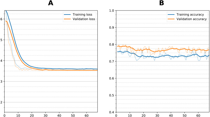
Results: The sequential convolutional approach yielded slightly better performance than the residual-based architecture, the zero-shot transfer learning approach yielded better performance than fine tuning, and CNN using longitudinal data performed better than CNN using a single timepoint MRI in predicting MCI conversion to AD. The best CNN model for predicting MCI conversion to AD at three years after diagnosis yielded a balanced accuracy of 0.793. Heatmaps of the prediction model showed regions most relevant to the network including the lateral ventricles, periventricular white matter and cortical gray matter.

Conclusions: This is the first convolutional neural network model using longitudinal and whole-brain 3D MRIs without extracting regional brain volumes or cortical thicknesses to predict future MCI to AD conversion at 3 years after diagnosis. This approach could lead to early prediction of patients who are likely to progress to AD and thus may lead to better management of the disease.

Keywords: Artificial intelligence; Convolutional neural networks; Dementia; Machine learning; Magnetic resonance imaging; Neuroimaging.

Figure 1. Overview of experimental design.

AD and NC MRI data were first trained to obtain weights (a classification task) for transfer learning (blue). After training, the weights are transferred to the prediction task (green) to predict whether patients will remain stable or progress within three years. Two different transfer learning methods were studied. With zero-shot, no further training was performed after the transfer, so the MCI images were analyzed for prediction by the network with the same weights copied over from the classification task. With fine-tuning, after weights are copied over from the classification task for initialization, additional training is performed against the MCI image data.

Figure 2. Single and dual time point CNN architecture.

(A) Single timepoint CNN. For classification, input consisted of a single timepoint full-subject 3D MRI of patients diagnosed at baseline as either AD or CN, and output was binary classification of AD vs CN. For prediction, input was a single timepoint full-subject 3D MRI of patients diagnosed as MCI and output was a binary prediction of whether the patient progressed (pMCI) or remained stable (sMCI) 3 years later. (B) Dual timepoint CNN. Input included 3D MRI images obtained at both baseline and 12 months, with the patient population and output categories identical than those used for single timepoint for classification and prediction. Both kinds of networks began with a series of convolutional blocks, followed by flattening into one or more fully connected layers ending in a final binary choice of classification or prediction.

Figure 3. Sequential, residual with bottleneck, and wide residual CNN blocks.

The convolutional layers portion of the network was organized as a series of blocks, each one with an increasing number K of activation maps (width), and with a corresponding decrease in resolution obtained by either pooling or stride during convolution. The figures detail the individual layers that compose a single block. (A) Sequential convolutional block. Each block was composed of a single 3 × 3 × 3 convolution, followed by batch normalization, ReLU activation, and max pooling to reduce the resolution. (B) Residual bottleneck with preactivation convolutional block. Convolutions were preceded by batch normalization and ReLU activation. Two bottleneck 3 × 3 × 3 convolutions have a width of K/4 followed by a final 1 × 1 × 1 convolution with K width. In parallel the skip residual used a 1 × 1 × 1 convolution to match the width and resolution. In this architecture the first residual block was preceded by an initial batch normalization followed by a single 5 × 5 × 5 convolution, plus one final batch normalization and ReLU activation after the last block (not shown). (C) Wide Residual Network convolutional block. In this architecture the batch normalization and activations occured after the convolutional layers. Each block had two 3 × 3 × 3 convolutional layers with 3D spatial dropout in between, plus a 1 × 1 × 1 skip residual convolution to match width and resolution.

Figure 4. Three head architectures.

(A) 3D global maximum pooling fully connected block. The global pooling inherently flattened the nodes into a fully connected layer with N nodes directly followed by the final binary classifier layer. (B) Long fully connected block. After flattening into a layer of N nodes, there are two sets of fully connected (size 2,048 and 1,024), batch normalization, and leaky ReLU activation layers separated by a single dropout layer, before the final binary classifier. (C) Medium fully connected block. Initial 3D max pooling is followed by flattening into a fully connected layer of size N followed by an additional fully connected layer of size 128 and ReLU activation.

Figure 5. Training curves during classification.

Loss and Accuracy curves during training for both training and validation sets. For sequential network and single timepoint, (A) loss, (B) accuracy. For wide residual network and dual timepoints, (C) loss, (D) accuracy. Solid lines are smoothed with 0.8 factor and faint lines show the unsmoothed values for each epoch.

Figure 6. Training curve during fine tuning for prediction.

(A) Loss function per epoch and (B) accuracy per epoch) during transfer learning fine tuning (sequential dual channel). Weights were initialized after training with AD vs. NC and then frozen at the convolutional layers, then additional training performed with the sMCI vs. pMCI data. There is an initial reduction in loss which stabilizes after 10 epochs, with no increase in accuracy.

Figure 7. (A-J) Heatmap visualization for 10 patients.

3D Grad-CAM heatmaps from the wide residual dual channel network used to predict conversion of MCI to AD. Heat maps were superimposed on individual patient’s anatomical MRI of 10 patients. A areas in bright yellow-orange (low to high) color corresponding to voxels with the gradient based on 3D Grad-CAM algorithm at the convolutional layer around 20 pixel resolution.