A brief introduction to the analysis of time-series data from biologging studies

Abstract

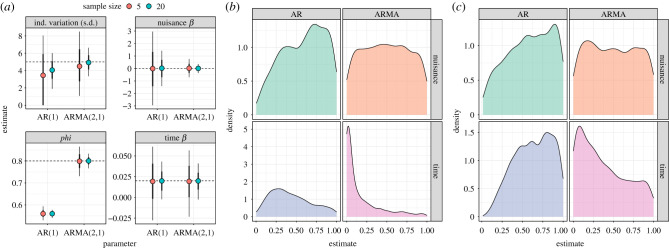
Recent advances in tagging and biologging technology have yielded unprecedented insights into wild animal physiology. However, time-series data from such wild tracking studies present numerous analytical challenges owing to their unique nature, often exhibiting strong autocorrelation within and among samples, low samples sizes and complicated random effect structures. Gleaning robust quantitative estimates from these physiological data, and, therefore, accurate insights into the life histories of the animals they pertain to, requires careful and thoughtful application of existing statistical tools. Using a combination of both simulated and real datasets, I highlight the key pitfalls associated with analysing physiological data from wild monitoring studies, and investigate issues of optimal study design, statistical power, and model precision and accuracy. I also recommend best practice approaches for dealing with their inherent limitations. This work will provide a concise, accessible roadmap for researchers looking to maximize the yield of information from complex and hard-won biologging datasets. This article is part of the theme issue 'Measuring physiology in free-living animals (Part II)'.

Keywords: animal movement; animal physiology; mixed models; temporal autocorrelation; time-series model.

Figure 1.

The effect of model specification on rates of Type I error when investigating differences in biologging data taken from two V. mongoliensis individuals. (a) Time-series traces of physiological measurements of two individual Velociraptors with identical means (μ = 0) and data-generating processes (AR1, rho = 0.5). (b) Densities of p-values from 1000 replicate iterations of data generation. Panel labels refer to analytical model (e.g. GLM) followed by term being tested (e.g. identification (ID)). Both GLMs and t-tests incorrectly estimate a significant difference between individuals in roughly 25% of simulations, well above the nominal α = 0.05. GLMs also incorrectly estimate a significant trend over time in greater than 25% of cases. Only GLS models accounting for temporal autocorrelation show the expected uniform distribution of p-values compatible with a Type I error rate controlled at 5%.

Figure 2.

Time-series data and model output of a real physiological dataset on beaver body temperature. (a) Beaver body temperature data from a single individual recorded every 10 min over approximately 24 h. (b) Modelling these data using a GLS model with a basic AR(1) temporal autocorrelation structure produces notable issues, namely a value of phi (estimate of the correlation strength between consecutive measures/10 min time steps) of 0, when there is a clear serial dependence structure (a). Importantly, autocorrelation plots of the residuals as in (b) help us identify that there is still unmodelled autocorrelation in these data. (c) Applying a more complex temporal autocorrelation model (ARMA(2,0)) resolves these issues and produces non-zero estimates parameters such as phi, as well as satisfactory autocorrelation plots. This shows us that we cannot always assume fitting a model allowing for temporal autocorrelation automatically deals with the signal of temporal autocorrelation in the data. Always check your model diagnostics for these tell-tale signs that something is not as it should be.

Figure 3.

Power analyses for physiological biologging studies. (a) Example data from loggers recording time-series depth data of five female (i) and five male (ii) fish. Different coloured traces denote different individuals. The data-generating process assumed a 20 m difference in the average dive depth between sexes, with equal variance of each sex, and an AR(1) temporal autocorrelation structure in the data with rho = 0.5. (b) Power curve of sample size versus expected statistical power for detecting the differences in dive depth between males and females. The x-axis denotes increasing sample size per sex (x = 5 represents a total sample size of 10 deployed (and retrieved!) loggers). These data show that we would need at least 35 loggers per sex to reach the threshold of 80% power at the assumed effect size. A larger difference between the sexes in the mean dive depth would probably require fewer loggers to be deployed. The key here is to be aware of the smallest meaningful difference you wish to detect and to conduct power simulations using that effect size before deploying any loggers.

Figure 4.

Effect of replication of random effects (number of individuals) on precision and accuracy of model estimates. (a) Time series of body temperature during flight for 10 individuals of a hypothetical shorebird species. Different colours represent different individuals. Data were generated using an AR(1) model with rho = 0.5 and the shape of the random effect distribution, representing true among-individual variation, had parameters μ = 40 and s.d. = 5. (b) Distribution of model estimates after 1000 replicate simulations for each value of individual sample size, ranging from 2 to 20. Different bar widths represent 66 and 95% intervals of the parameter distributions. At low individual/random effect replication (less than 10), both accuracy and precision of the estimate of among-individual variation are compromised (true s.d. value 5, dashed line). Above 10 ‘levels’ of the random effect, estimates stabilize in both accuracy and precision. The estimation accuracy of the autocorrelation parameter is uniform for all sample sizes on average, but precision suffered at values n < 8. Collectively, these data show that even if autocorrelation is being ‘dealt with’ by the models, the resulting parameter estimates may be quite unreliable if random effect sample sizes are low.

Figure 5.

The effect of model structure and sample size on model accuracy. Data were generated using an ARMA(2,1) autocorrelation structure with sample size (number of individuals) of 5 or 20 and 100 values per time series. Model fitting used either a simple AR(1) or ARMA(2,1) correlation structure, i.e. the latter was the data-generating model. All models contained an effect of time (β = 0.02) and included a nuisance variable (nuisance) with no effect on the outcome (β = 0). (a) Parameter estimates after 1000 replicate simulations for each sample size and correlation structure. Only the first phi parameter of the ARMA model is shown for comparison with the AR model (equivalent to rho). (b,c) The distributions of rho values for the two fixed effects (nuisance and time) derived from the summary tables, i.e. based on Wald tests for n = 20 (b) and n = 5 (c). Note this is not a formal test of a variable's ‘significance’ through model selection, but gives a good indication of the model's assumed precision of the estimate.

References

-
- Hawkes LA, Exeter O, Henderson SM, Kerry C, Kukuluya A, Rudd J, Whelan S, Yoder N, Witt MJ. 2020. Autonomous underwater videography and tracking of basking sharks. Anim. Biotelemetry 8, 29. (10.1186/s40317-020-00216-w) - DOI
- Smith BJ, Hart KM, Mazzotti FJ, Basille M, Romagosa CM. 2018. Evaluating GPS biologging technology for studying spatial ecology of large constricting snakes. Anim. Biotelemetry 6, 1. (10.1186/s40317-018-0145-3) - DOI
Publication types
MeSH terms
LinkOut - more resources
Full Text Sources