Topological data analysis distinguishes parameter regimes in the Anderson-Chaplain model of angiogenesis

Abstract

Angiogenesis is the process by which blood vessels form from pre-existing vessels. It plays a key role in many biological processes, including embryonic development and wound healing, and contributes to many diseases including cancer and rheumatoid arthritis. The structure of the resulting vessel networks determines their ability to deliver nutrients and remove waste products from biological tissues. Here we simulate the Anderson-Chaplain model of angiogenesis at different parameter values and quantify the vessel architectures of the resulting synthetic data. Specifically, we propose a topological data analysis (TDA) pipeline for systematic analysis of the model. TDA is a vibrant and relatively new field of computational mathematics for studying the shape of data. We compute topological and standard descriptors of model simulations generated by different parameter values. We show that TDA of model simulation data stratifies parameter space into regions with similar vessel morphology. The methodologies proposed here are widely applicable to other synthetic and experimental data including wound healing, development, and plant biology.

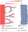
Fig 1. Schematic overview of tumor-induced angiogenesis.

Schematic depicting seven aspects angiogenesis that are incorporated in the Anderson-Chaplain model of tumor-induced angiogenesis [17]. (1) Distant tumor cells release a range of chemoattractants, including vascular endothelial growth factors and basic fibroblast growth factors that stimulate the formation of new blood vessels. These growth factors are described collectively as a single, generic tumor angiogenesis factor (TAF). (2) Production and consumption of tissue-matrix bound fibronectin by the endothelial cells creates a spatial gradient of fibronectin across the domain. (3) Endothelial cells sense the TAF and fibronectin gradients and undergo individual cell migration. (4) As endothelial tip cells migrate, via chemotaxis, up spatial gradients of the TAF, stalk cells in the developing vessels are assumed to proliferate, creating what has been termed a “snail trail” of new endothelial cells. (5) Endothelial tip cells also migrate, via haptotaxis, up spatial gradients of fibronectin. (6) Endothelial cells in existing sprouts may initiate the formation of secondary sprouts. (7) If a sprout coincides with an existing vessel, then it is assumed to be annihilated and a new loop is formed; if two sprouts coincide or anastomose, then both are assumed to be annihilated and a new loop forms.

Fig 2. Data generation and analysis pipeline.

(1) Spatio-temporal modeling: Anderson-Chaplain model. The Anderson-Chaplain model is simulated for 11 × 11 = 121 different values of the haptotaxis and chemotaxis parameters, (ρ, χ). The model output is saved as a binary image, where pixels labeled 1 or 0 denote the presence or absence, respectively, of blood vessels. We generate 10 realizations for each of the 121 parameter combinations, leading to 1,210 images of simulated vessel networks. (2) Data analysis. We use the binary images from Step 1 to generate standard and topological descriptor vectors A.) Standard descriptor vectors We compute the number of active tip cells and the number of vessel segments at discrete time points. We also compute the length of the vessels at the final time point [32, 34, 35, 52]. B.) Topological descriptor vectors. We construct flooding and sweeping plane filtrations [44] using binary images from the final timepoint of each simulation. We track the birth and death of topological features (connected components and loops) that are summarized as Betti curves and persistence images [52]. (3) Data clustering. We perform k-means clustering using either the standard or topological descriptor vectors computed during step 2 from all 1,210 simulations. In this way, we decompose (ρ, χ) parameter space into regions that group vessel networks with similar morphologies.

Fig 3. Standard descriptor overview.

Standard descriptors are computed for each model simulation include the number of vessel segments (N_S, depicted by each colored solid curve), the number of endothelial tip cells (N_T, depicted by black dots), and the x-coordinate of the vessel segment location with the greatest horizontal distance from the y-axis (L, depicted by the vertical grayed dashed line). This schematic example is initialized with 2 vessel segments and 2 tip cells at locations (1) and (2). A branching event at location (3) increases the value of both N_S and N_T by one. An anastomosis event at location (4) decreases N_T by one. The branching event at location (5) increases both N_S and N_T by one.

Fig 4. Converting a binary image into a simplicial complex.

A) Schematic binary image. B) Point cloud for all nonzero pixels in the binary image. The Moore neighborhood of one nonzero pixel is highlighted in salmon. C) A simplicial complex constructed from the point cloud in panel B.

Fig 5. The LTR sweeping plane filtration for a binary image.

A) Sample binary image from a simulation of the Anderson-Chaplain model. B-E) Point clouds used for each iteration of the sweeping plane approach. On each step, only pixels located to the left of the plane (denoted here with a blue line) are included; gray pixels are ignored. F-I) Filtration steps constructed from the point clouds in panels B-E.

Fig 6. The flooding filtration for a binary image.

A) Schematic binary image. B) Grayscale image of the original binary image. Red pixels are nonzero in the initial image, orange pixels become nonzero after one round of flooding, and yellow pixels become nonzero after two rounds of flooding. C-E) We performed three filtrations by dilating the image twice. During each filtration, the eight neighboring pixels of all nonzero pixels (ie pixels not marked as white) become nonzero. Red pixels are nonzero in the original image, orange pixels become nonzero on the second filtration (i.e., after one step of flooding), and yellow pixels become nonzero on the third filtration (i.e., after two steps of flooding). F-H) Simplicial complexes associated with the filtrations presented in panels C-E.

Fig 7. Typical realizations of the Anderson-Chaplain model.

A) Chemotaxis-driven tip cell movement (ρ = 0.00, χ = 0.50), B) haptotaxis-driven tip cell movemement (ρ = 0.50, χ = 0.00), and C) tip cell movement driven by chemotaxis and haptotaxis (ρ = 0.15, χ = 0.15).

Fig 8. Standard and topological descriptors describe distinct aspects of vessel morphology.

For clarity, each vessel segment is colored differently, and black dots represent active tip cells. A) The initial vessel configuration. B) A schematic showing how the vascular architecture changes after an anastomosis event. C) A schematic showing how the vascular architecture changes after a branching event. D-E) Schematics showing two ways in which vasculature can change after one anastomosis event and one branching event. F) A schematic showing how the vessels can change after one branching and two anastomosis events. (Key: β₀, number of connected components; β₁, number of loops; N_T, number of tip cells; N_S, number of vessel segments).

Fig 9. The standard descriptors used to summarize model simulations.

We show how the following descriptors change over 50 time steps for the three simulations presented in Fig 7: A) the number of tip cells, N_T(t), B) the number of vessel segments, N_S(t), and C) the final vessel length, L(t_end).

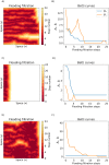
Fig 10. TDA sweeping plane descriptor vectors.

A) The sweeping plane directions are left-to-right (LTR, gray); right-to-left (RTL, orange); bottom-to-top (BTT, cyan); and top-to-bottom (TTB, green). For these four v = iTj filtrations, we started with points on the ith boundary and included more points as we stepped towards the jth boundary. Repeating this process produced the spatial filtration K^v = K₀, K₁…K_end for v = {LTR, RTL, TTB, BTT}. B-D) We formed the Betti curves β₀(K^v) and β₁(K^v) by computing the Betti numbers along each step of K^v for the three blood vessel simulations presented in Fig 7; B) the chemotaxis-driven simulation, C) the haptotaxis-driven simulation and D) chemotaxis and haptotaxis simulation.

Fig 11. The flooding filtration.

A,C,E) Illustrate the flooding filtrations for the three blood vessel simulations from Fig 7. Dark red pixels were points included in the first steps of the filtration and yellow pixels were the points included in later filtration steps. White pixels were not included after 24 steps of the flooding filtration. B,D,F) The Betti Curves (β₀(K^flood) and β₁(K^flood)) for the chemotaxis-driven, haptotaxis-driven, and chemotaxis and haptotaxis simulations respectively.

Fig 12. Partitioning (ρ, χ) parameter space into distinct regions using standard biological descriptor vectors.

We applied k-means clustering, with k = 5, to standard biological descriptor vectors. The resulting partitions are presented for A) N_T(t), B) N_S(t), C) L(t_end), and D) concatenation of all three descriptor vectors. The five clusters are ordered according to the mean χ value within the cluster.

Fig 13. Partitioning (ρ, χ) parameter space into distinct regions using sweeping plane double descriptor vectors.

We applied k-means clustering, with k = 5, to sweeping plane double descriptor vectors. The resulting partitions are presented for the four descriptor vectors that have the highest OOS accuracy: A) PIO₀(K^LTR) & PIO₀(K^RTL), B) PIO₀(K^RTL) & PIR₁(K^LTR), C) PIO₀(K^TTB) & PIR₁(K^LTR), and D) PIO₀(K^BTT) & PIR₁(K^LTR). The five clusters are ordered according to the mean χ value within the cluster.

Fig 14. Representative simulated blood vessel networks from Groups 1–5.

Series of simulations that resemble the means from each of the five groups (as identified from the double descriptor vectors associated with the sweeping plane filtrations PIO₀(K^LTR) & PIO₀(K^RTL)). The representative simulations for groups 1–5 were generated using the following pairs of parameter values: (ρ, χ) = (0.25, 0), (0.5, 0.2), (0.3, 0.2), (0.15, 0.15), and (0.2, 0.4), respectively.

References

1. Gupta MK, Qin RY. Mechanism and its regulation of tumor-induced angiogenesis. World Journal of Gastroenterology. 2003;9(6):1144–1155. doi: 10.3748/wjg.v9.i6.1144 - DOI - PMC - PubMed
1. Kushner EJ, Bautch VL. Building blood vessels in development and disease. Current Opinion in Hematology. 2013;20(3):231–236. - PubMed
1. Tonnesen MG, Feng X, Clark RAF. Angiogenesis in wound healing. Journal of Investigative Dermatology Symposium Proceedings. 2000;5(1):40–46. doi: 10.1046/j.1087-0024.2000.00014.x - DOI - PubMed
1. Ferrara N. VEGF and the quest for tumour angiogenesis factors. Nature Reviews Cancer. 2002;2(10):795–803. doi: 10.1038/nrc909 - DOI - PubMed
1. Folkman J. Tumor angiogenesis. In: Klein G, Weinhouse S, Haddow A, editors. Advances in Cancer Research. vol. 19. Academic Press; 1974. p. 331–358. - PubMed
Publication types