Causal role for the primate superior colliculus in the computation of evidence for perceptual decisions

Abstract

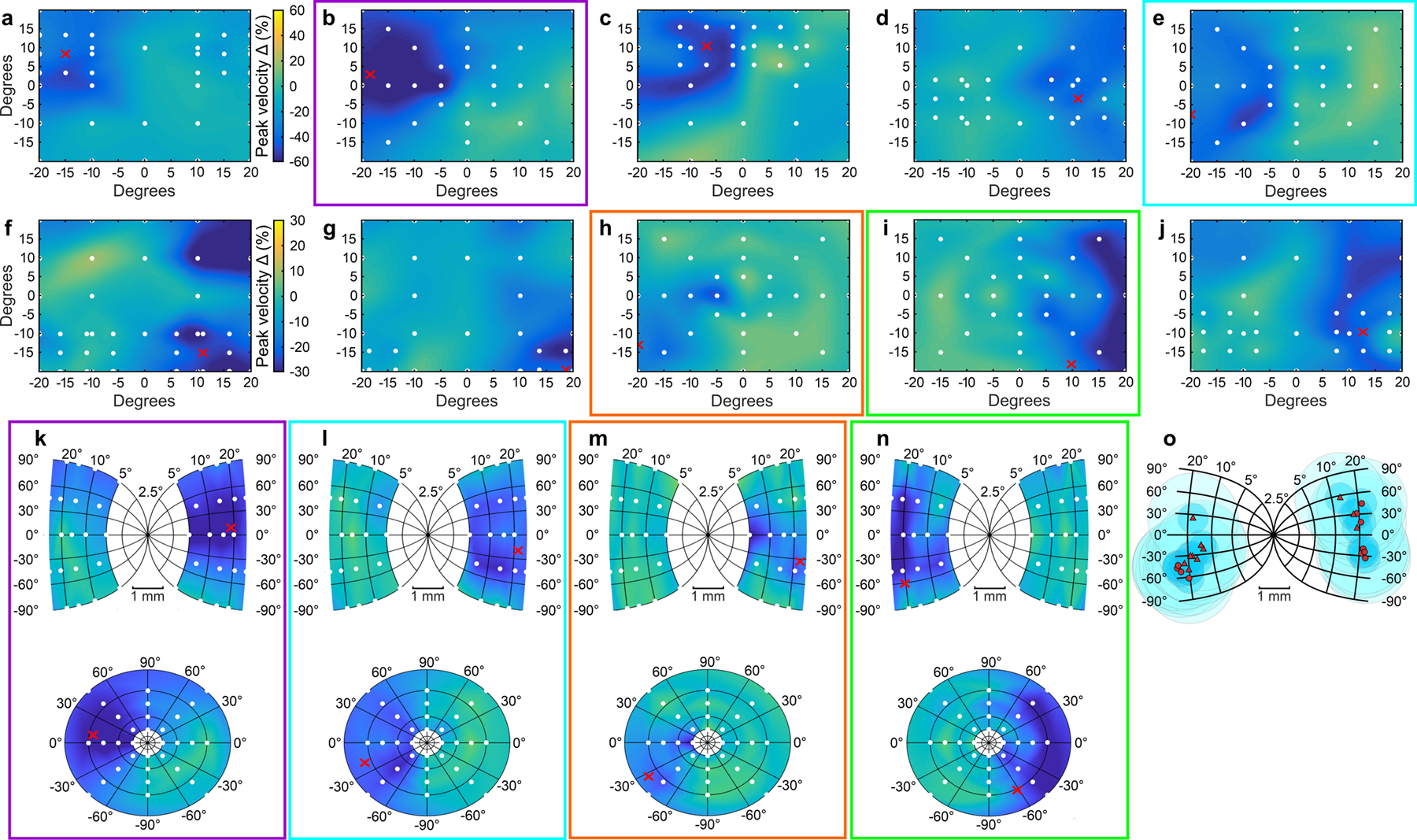
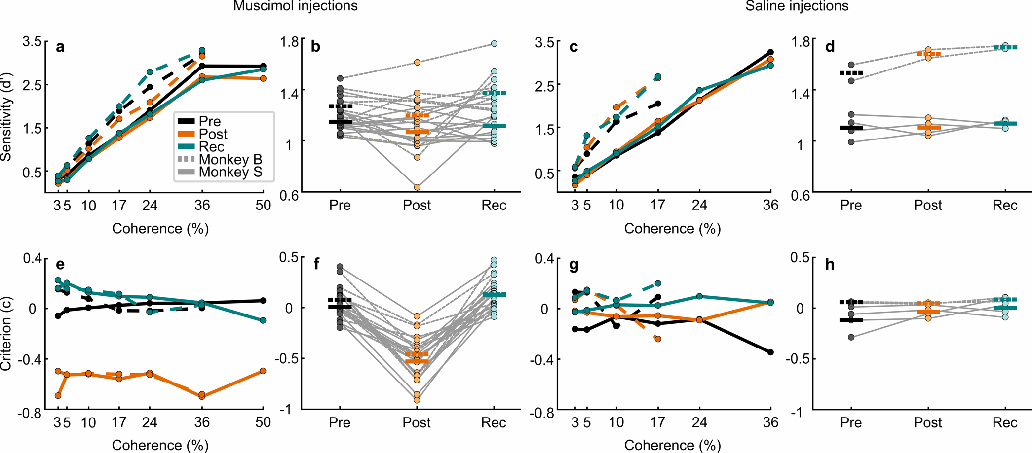
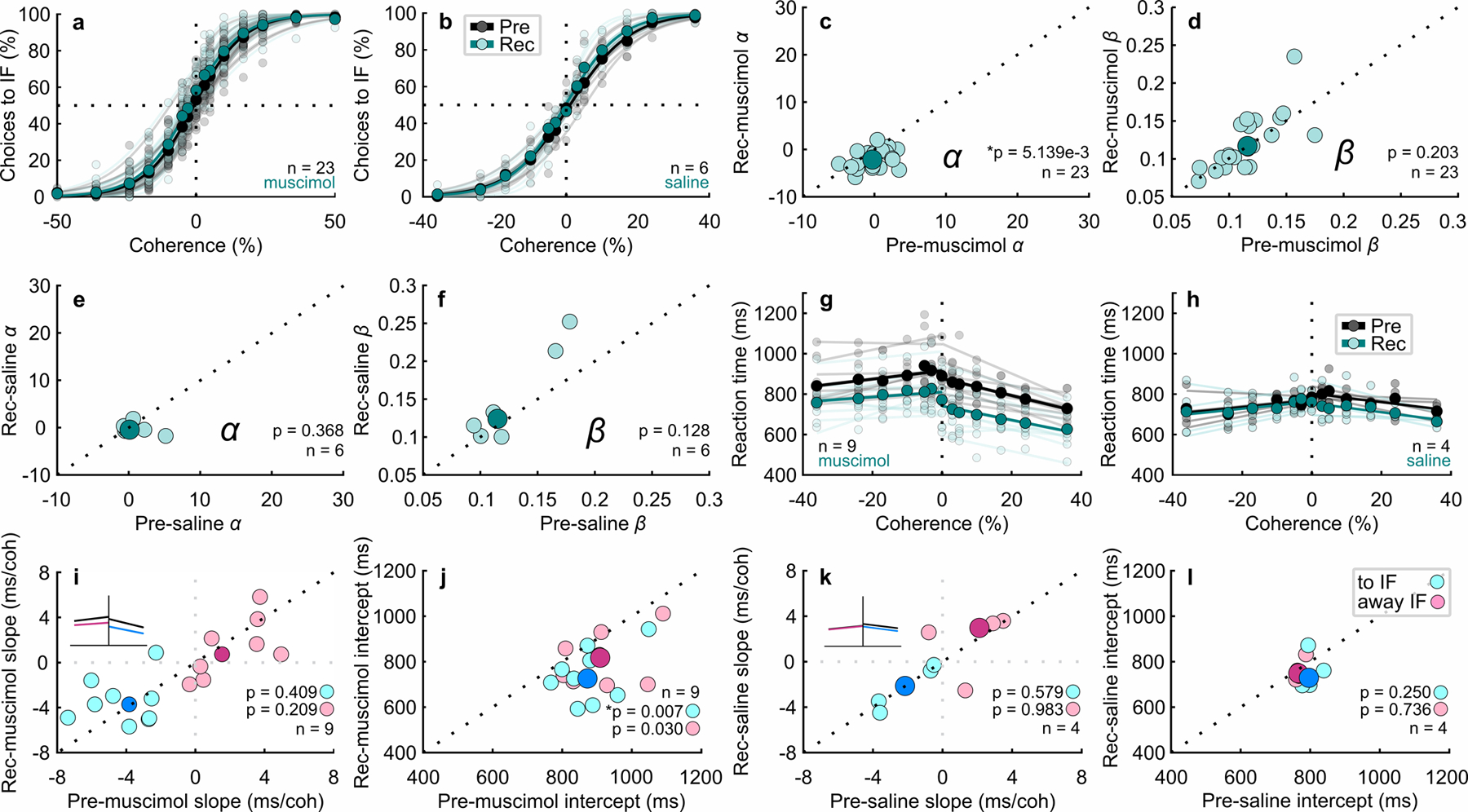
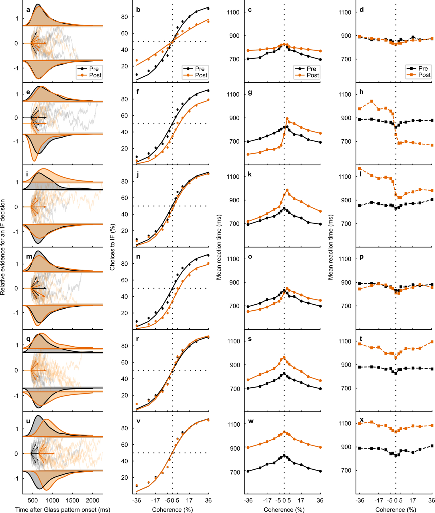
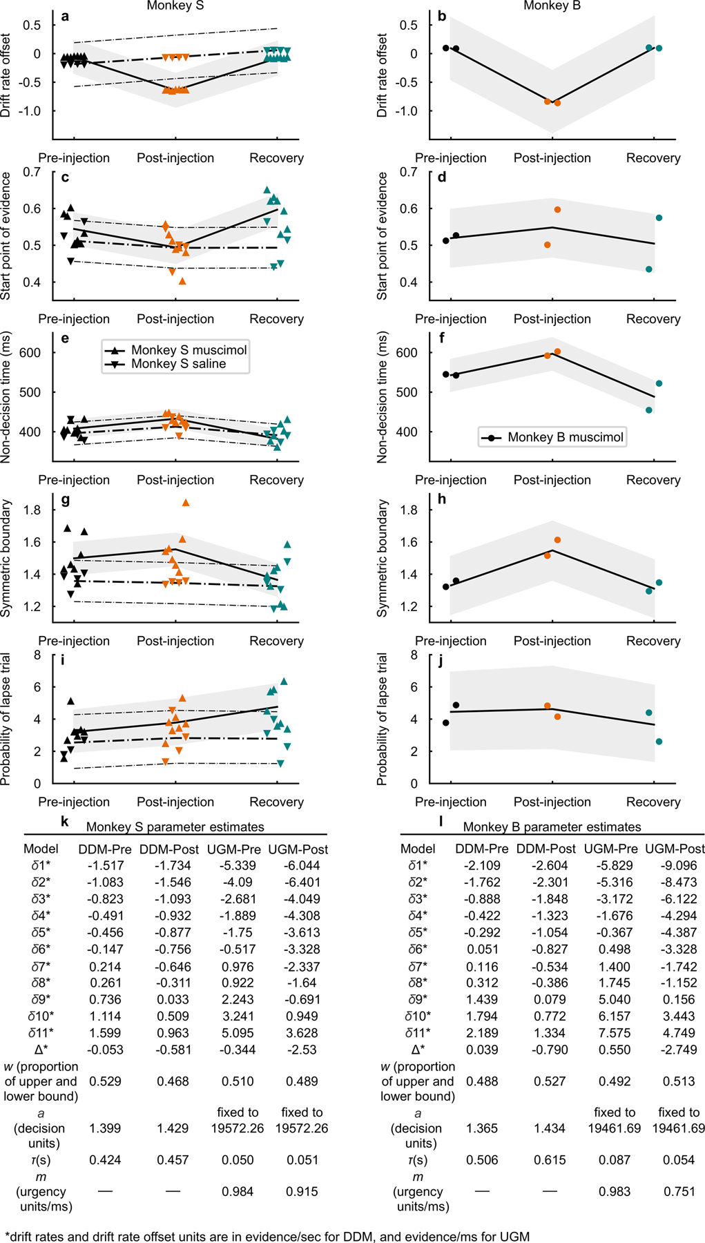
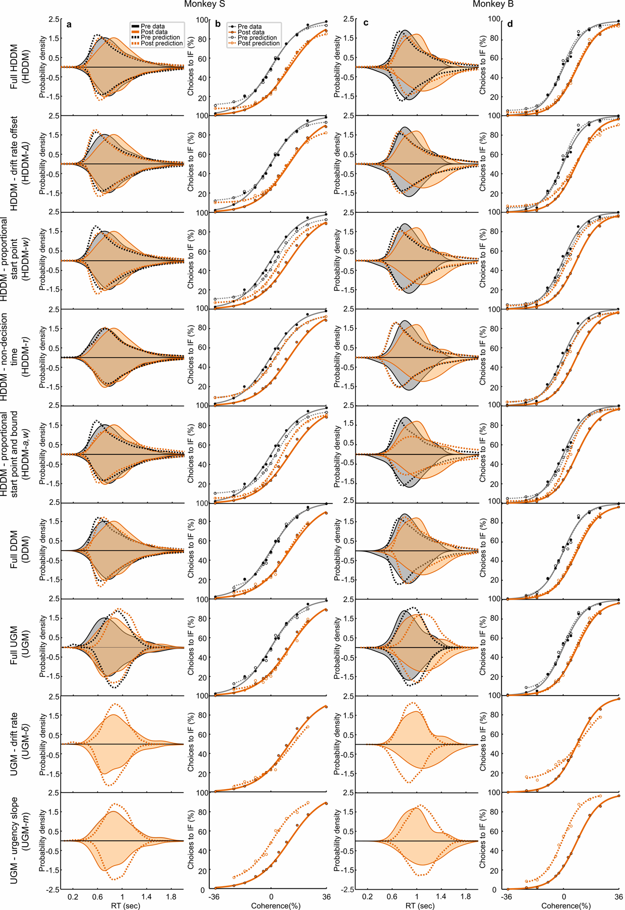
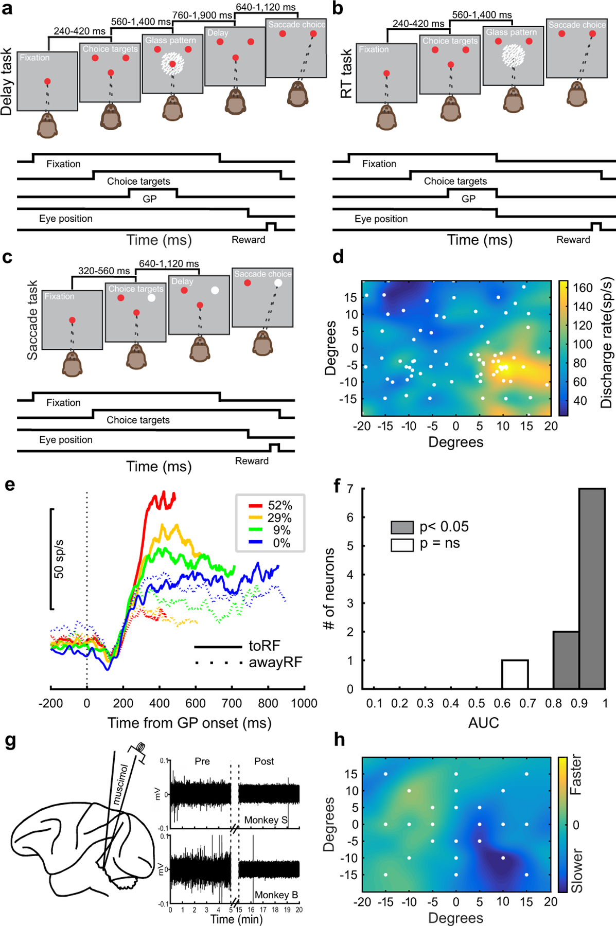
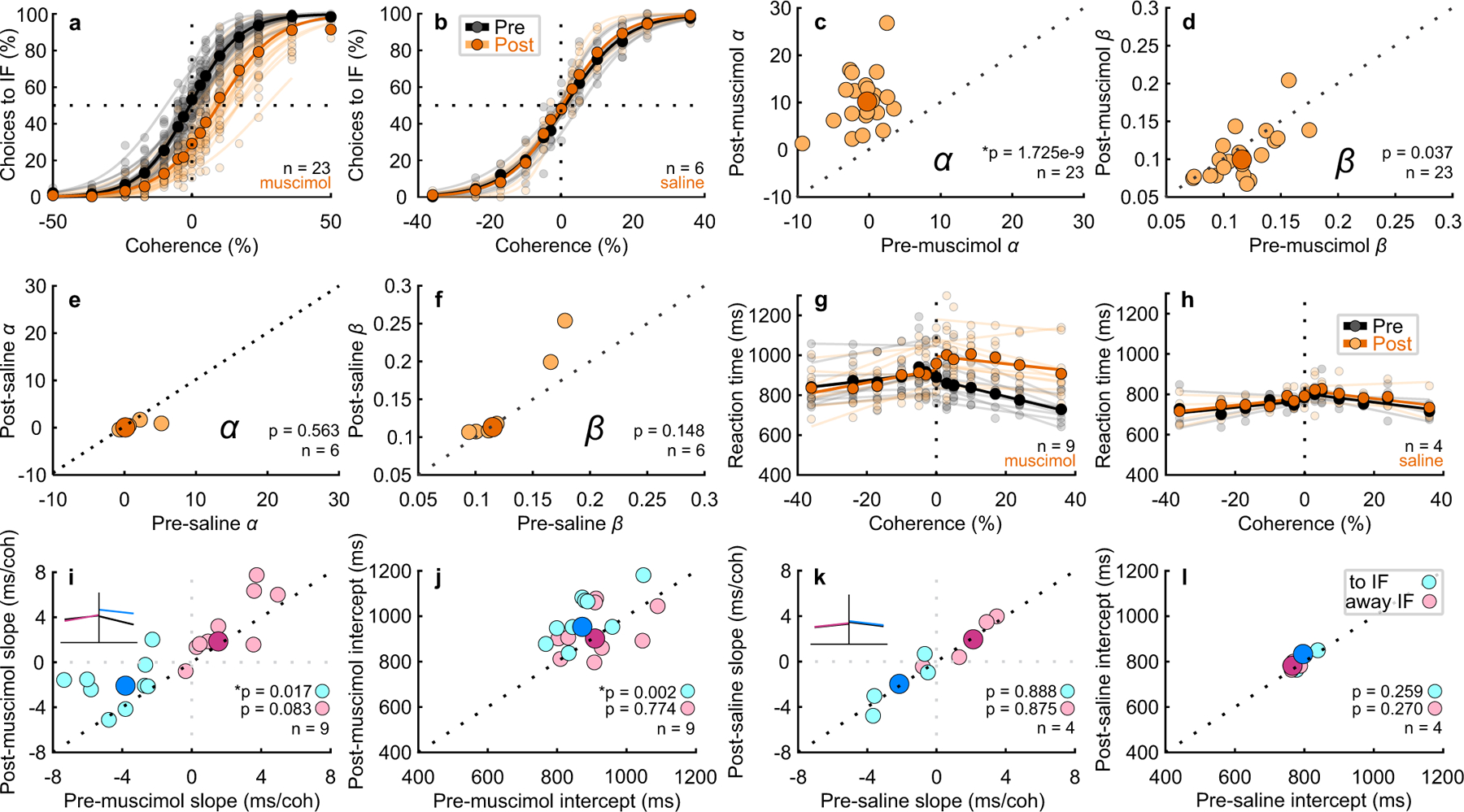
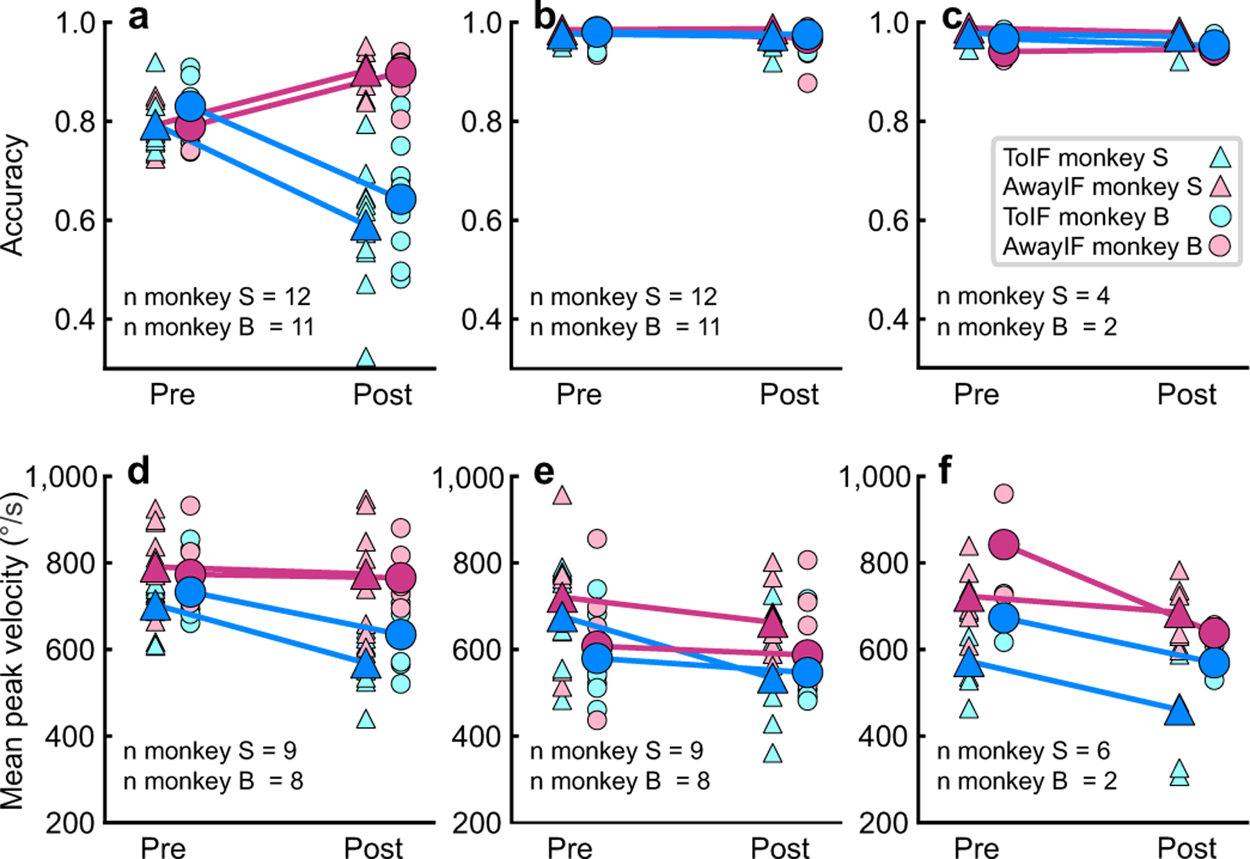
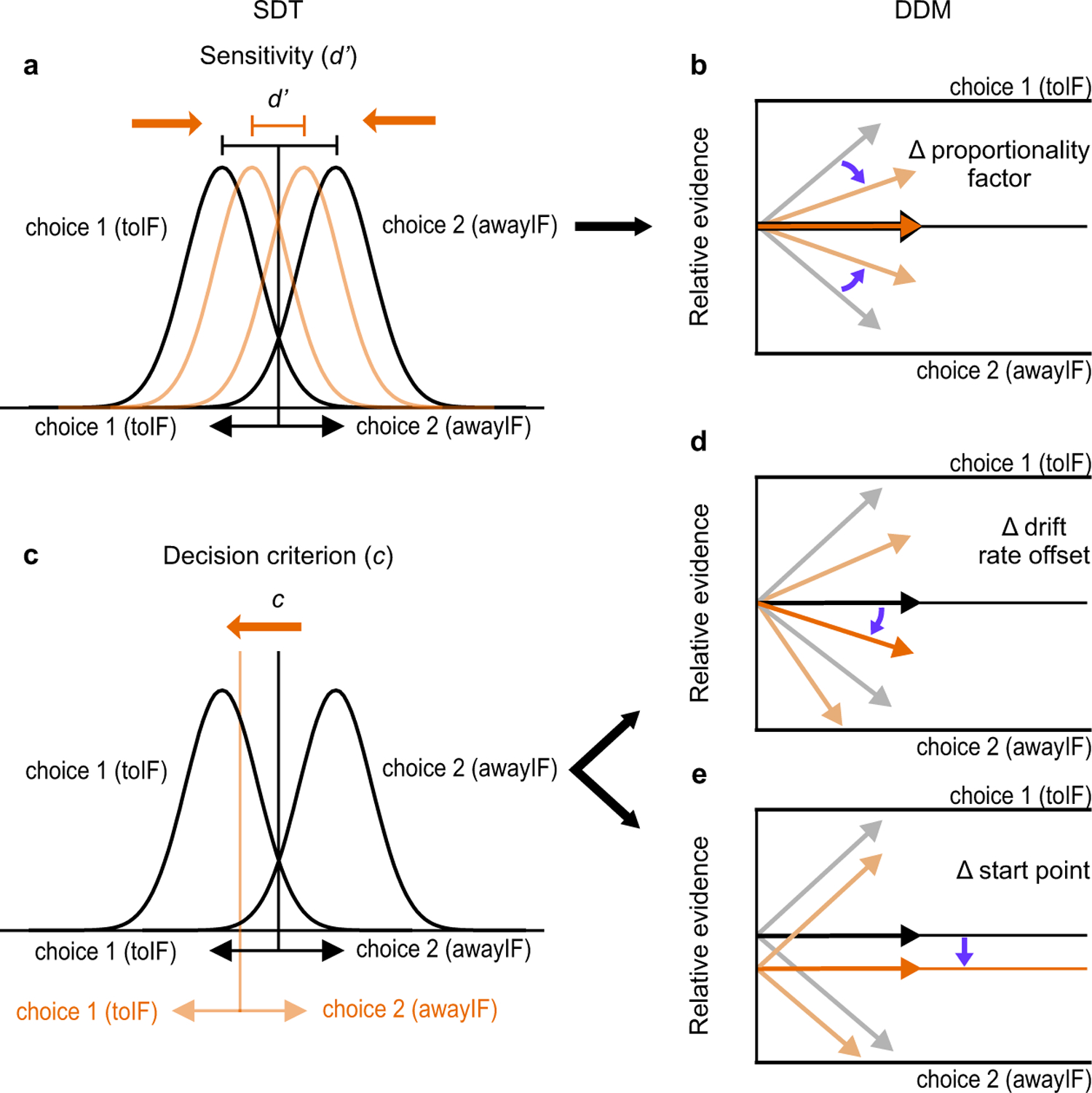
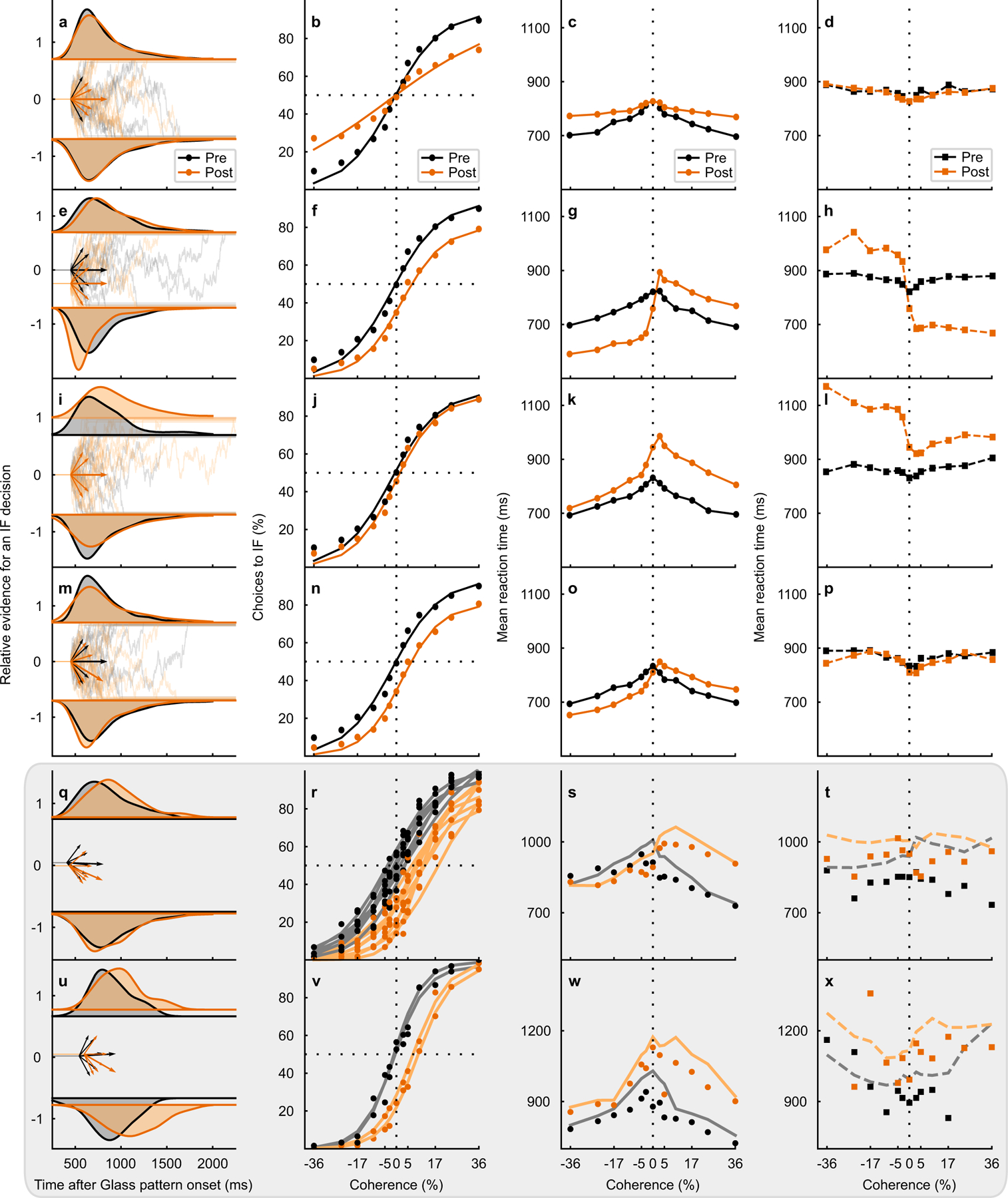
Trained monkeys performed a two-choice perceptual decision-making task in which they reported the perceived orientation of a dynamic Glass pattern, before and after unilateral, reversible, inactivation of a brainstem area-the superior colliculus (SC)-involved in preparing eye movements. We found that unilateral SC inactivation produced significant decision biases and changes in reaction times consistent with a causal role for the primate SC in perceptual decision-making. Fitting signal detection theory and sequential sampling models to the data showed that SC inactivation produced a decrease in the relative evidence for contralateral decisions, as if adding a constant offset to a time-varying evidence signal for the ipsilateral choice. The results provide causal evidence for an embodied cognition model of perceptual decision-making and provide compelling evidence that the SC of primates (a brainstem structure) plays a causal role in how evidence is computed for decisions-a process usually attributed to the forebrain.

Extended Data Fig. 1. Estimates of muscimol spread in the SC

(Associated with Fig. 1 main text) a–j The reduction in peak velocity from pre- to post-muscimol for 10 muscimol injections (four from monkey B, six from monkey S), one to two hours post injection. The percent change in peak velocity after muscimol injection (post-muscimol saccade velocity minus pre-muscimol saccade velocity divided by pre-muscimol saccade velocity multiplied by 100), is plotted for the target positions indicated by the white circles and linearly interpolated on the visual field in Cartesian coordinates. Cooler colors indicate slower saccadic velocities post-muscimol. a–e shows five injections with more concentrated effects of muscimol (color bar scaled from −60% to 60%), whereas f–j shows five injections with smaller but more diffuse effects of muscimol (color bar scaled from −30% to 30%), showing the range in the efficacy of our muscimol injections based on changes in saccade velocity at least one hour post injection. Red Xs show the site of injection based on the RF determined electrophysiologically (Supplementary Table 1). The peak velocity maps highlighted by the colored boxes in a–j had a uniform and homogenous sampling of positions in the visual field that allowed us to calculate the estimated spread across the SC map as shown in k–n (Quaia, C., Aizawa, H., Optican, L.M. & Wurtz, R.H. Reversible inactivation of monkey superior colliculus: II. Maps of saccadic deficits. Journal of Neurophysiology 79, 2097–2110 (1998).). k–n show the same percent change in peak velocity after muscimol injections plotted on the SC map (top) and the visual field in polar coordinates (bottom) for the injections in the corresponding colored boxes in a–j. o shows the locations of muscimol injections and spread estimates plotted onto the SC map. Red circles show injection locations for monkey B and red triangles show injections from monkey S. Each injection’s estimated muscimol spread is represented by two concentric circles. The darker shaded circles show 0.5 mm radius and the lighter shaded circles shows 1.5 mm radius from the center of the injection site based on estimates from (Allen, T.A., et al. Imaging the spread of reversible brain inactivations using fluorescent muscimol. Journal of Neuroscience Methods 171, 30–38 (2008).). There were three injections in which muscimol may have spread into the pretectal region and thus also the foveal region of the rostral SC, as evidenced by the occurrence of ocular nystagmus about an hour after the injection. In these cases, we aborted the experiment and omitted the data from analyses upon appearance of nystagmus. One example appears in b and k (maps highlighted by purple boxes). The Glass pattern decision and selection task data before the occurrence of nystagmus are included in the analysis in the main text. The effect on the psychometric function from this example was the largest that we observed (Fig. 2a, rightmost transparent orange psychometric function).

Extended Data Fig. 2. AIC and BIC scores for the two, three and four parameter logistic function fits

(Associated with Fig. 2 of the main text) a AIC scores for each pre- and post-injection and recovery sessions for all muscimol and saline injections (n=87 sessions) for two, three, and four parameter logistic fits to the performance data. The circles show the AIC score of the logistic fit to each individual session from the n=87 total sessions (pre-, post- and recovery * 29 injections), and the black, horizontal bars show the mean AIC score. The dotted lines connect the same data sessions that were fit across the two, three, and four parameter fits to see if there were any changes in AIC score between the fits with different number of parameters. The two parameter logistic model has two parameters: α (decision bias) and β (sensitivity) following the equation p(IF) = 1/(1+exp(−β(k-α))) (Eq 1 in Methods), which was used to fit the psychometric functions in Fig. 2 and Extended Data Fig. 4. The three parameter logistic model includes: α, β, and ʎ (lapse rate or the difference between perfect performance and the top and bottom asymptotes) following the equation p(IF) = ʎ + (1–2ʎ)/(1+exp(−β(k-α))). The four parameter logistic model includes: α, β and ʎ (lapse rate or the difference in perfect performance and asymptotic performance for toIF decisions) and γ (lapse rate or the difference in perfect performance and asymptotic performance for awayIF decisions) following the equation p(IF) = γ + (1-γ-λ)/(1+exp(−β(k-α))). When looking at the AIC scores for the two, three, and four parameter fits (lower AIC scores indicate a better fit given model complexity), we see that the data are explained equally well or better with the models without lapse rates, with mean scores of 638.80 for the two parameter fit, 640.51 for the three parameter fit, and 641.47 for the four parameter fit. Therefore, we selected the simpler, two parameter model to fit the performance data. b Same as in a for the BIC scores, with mean of 639.93 for the two parameter fit, 642.20 for the three parameter fit, and 643.73 for the four parameter fit. The lack of difference in the quality of the fits with or without the lapse rate parameters is consistent with the parameter estimation results of lapse rates in the hierarchical DDM (Extended Data Fig. 6i,j).

Extended Data Fig. 3. Decision criterion but not sensitivity, is impacted by unilateral SC inactivation during one-interval, two-choice perceptual decision-making

(Associated with Fig. 2 main text) a Sensitivity, as measured by d’ is plotted against coherence for all experiments from both monkeys pre-muscimol (black circles and lines), post-muscimol (orange circles and lines) and 24 hour recovery (green circles and lines). Dashed lines show data from monkey B and solid lines show data from monkey S. Note that for monkey S, there is an additional 50% coherence condition (Methods). Qualitatively, monkey B showed a higher sensitivity for the same Glass pattern coherences than monkey S. b d’ collapsed over coherence and plotted for pre-muscimol (grey circles), post-muscimol (orange circles) and recovery (green circles) for all experiments from both monkeys. Dashed lines show data from monkey B (n=11 injections) and solid lines show data from monkey S (n=12 injections). The horizontal lines indicate the mean d’ across sessions. On average there were no significant changes in d’ with muscimol in either monkey (monkey S, t(11) = −1.54, p = 0.152, 95% CI = [−0.23, 0.07]; monkey B, t(10) = −1.51, p = 0.161, 95% CI = [−0.21, 0.07]). c–d Same as in a and b for the saline injections. Because we only had two saline injections in monkey B, we collapsed the data across monkeys (n=6 injections) for statistical analysis, but the data are shown separated by monkey. We found no significant differences in d’ with saline (t(5) = 1.20, p = 0.283, 95% CI = [−0.1, 0.19]). Note that there are no d’ or criterion (c) values for monkey B for the 24% and 36% coherences due to a lack of errors for the awayIF post-muscimol 24% and 36% coherence trials. e Criterion (c) plotted against coherence for pre-muscimol (black), post-muscimol (orange), and recovery (green) for all experiments from both monkeys. Dashed lines are from monkey B and solid lines are from monkey S. This plot is shown for symmetry with the d’ plot although criterion changes across coherences are not particularly meaningful as monkeys are not expected to change their criterion across coherences as the coherences were randomized from trial to trial and there was no way for the monkeys to know which coherence was impending. f Criterion collapsed over coherence plotted for pre-muscimol, post-muscimol and recovery for all experiments (n=12 injections for monkey S, n=11 injections for monkey B). For both monkeys, c changed significantly with muscimol (monkey S, t(11) = −9.34, p = 1.46 × 10 ⁻⁶, 95% CI = [−0.7, −0.38], monkey B, t(10) = −7.48, p = 2.10 × 10 ⁻⁵, 95% CI = [−0.75, −0.33]). g–h Same as in e-f for the saline experiments from both monkeys (n=6 injections). We found no significant differences in c with saline injections (w(5) = 18, p = 0.156). Consistent with the psychometric function results shown in Fig. 2, unilateral inactivation of SC with muscimol produced changes in decision bias and not perceptual sensitivity.

Extended Data Fig. 4. Decision-making behavior 24 hours after muscimol

(Associated with Fig. 2 of the main text) a Proportion of choices to the inactivated field (toIF) is plotted as a function of Glass pattern coherence. Black circles show pre-muscimol performance data and green circles show 24-hour recovery performance data. The black and green lines show the two parameter logistic fits to the performance data. n=23 injections. b Same as in a for the pre-saline (black circles and lines) and the 24-hour recovery from saline (green circles and lines). n=6 injections. c α parameters from the logistic fits for the recovery data (rec-muscimol) plotted against α parameters from the fits for the pre-muscimol data. On average, the α parameter shifted leftward during the recovery period compared to the pre-muscimol control (w(22) = 230, p = 0.005). Note that this was opposite to the direction of the shift that occurred post-muscimol as seen in the main Fig. 2a, as if the monkeys over-compensated for the effect of muscimol during recovery. d β parameters from the logistic fits for the recovery data plotted against the β parameters from the fits from the pre-muscimol data. On average, there were no significant differences in the β parameter (t(22) = −1.31, p = 0.20, 95% CI = [−0.02, 6.0 × 10⁻³]). e–f Same as in c and d for the saline experiments. g Reaction time (RT) plotted against coherence for the pre-muscimol data (black circles) and recovery data (green circles) from the RT version of the decision task (n=9 injections). The lines show linear fits to the RT data. The RT was shorter for the recovery data compared to the pre-muscimol data for all coherences. Similar to the results of the α parameter comparisons, the RT finding suggests a compensatory response to the muscimol injections 24 hours earlier. h Same as in g for the saline experiments. i The slope parameter from the linear fits to the RT data for the recovery data plotted against the pre-muscimol data. Cyan circles show the parameter of the linear fits of the RT data for toIF decisions (positive coherences) and magenta circles show the RT data for awayIF decisions (negative coherences). There were no significant differences on average (RT slope awayIF, t(8) = 1.37, p = 0.21, 95% CI = [−0.87, 2.59]; RT slope toIF, t(8) = −0.87, p = 0.41, 95% CI = [−3.10, 1.61]). j same as in i for the intercept parameter. There were significant changes in the intercept on average for the toIF side (RT intercept, t(8) = 3.61, p = 0.007, 95% CI = [32.55, 240.50]) but not the awayIF side (RT intercept, t(8) =2.63, p = 0.03 n.s. Bonferroni correction, 95% CI = [−4.89, 216.53]). k–l Same as in i and j for the saline experiments. There were no significant differences in slope or intercept for these experiments (RT slope awayIF, t(3) = −0.02, p = 0.98, 95% CI = [−6.26, 6.19]; RT slope toIF, t(3) = 0.62, p = 0.58, 95% CI = [−0.88, 1.19]; RT intercept awayIF, t(3) = 0.37, p = 0.74, 95% CI = [−71.20, 85.05]; RT intercept toIF, w(3) = 9, p = 0.25). Note that four saline experiments were performed in the RT task and the other two were performed using the delayed version of the task so only four observations appear in this plot. Note that the darker shaded symbols show the median values and the 95% confidence intervals are from the means.

Extended Data Fig. 5. DDM model simulations for changes in model parameters

(Associated with Fig. 4 and 5 of the main text). Panels a-p are the same as those shown in Fig. 5 of the main text. a RT distribution from the 0% coherence condition (density approximated through kernel smoothing) predicted by a DDM simulation with only decrease in proportionality factor between coherence and drift rate post-muscimol (orange). Pre-muscimol shown in black. Below the RT distributions, the relative evidence for toIF decisions is plotted over time since the Glass pattern onset and the short arrows show drift rates for toIF decisions (positive) and awayIF decisions (negative) pre- and post-muscimol, for the 0%, 10%, and 36% coherence conditions. The longer arrows show the mean drift rate across both toIF and awayIF directions and all coherences, termed drift rate offset b The psychometric function, plotted as a proportion of toIF choices over coherences, predicted by the DDM variant simulation with a decrease in proportionality factor between coherence and drift rate which changes the slope (without a shift) of the psychometric function. A change in the slope of the psychometric function was not observed in the data (Fig. 5r, v, shaded), making the decrease in proportionality factor between coherence and drift rate an unlikely explanation for the observed data. c Mean RT predictions for correct trials for each coherence condition for the DDM simulation with a decrease in proportionality factor between coherence and drift rate, for pre- (black) and post-muscimol (orange). d Same as in c but for error trials. e–h Same as in a-d but for the DDM variant simulation with only a change in proportional start-point of the evidence accumulation path away from the IF (often interpreted as an initial bias away from the IF). A decrease in proportional start point away from the IF predicts a shift in the psychometric function as observed in the real data (Fig. 5r,v, shaded), making a change in the proportional start point a possibility in explaining the decision bias we observed in the post-muscimol data. However, a start point change away from the IF also predicts a decrease in error toIF RTs which we did not observe in the data (Fig. 5t,x, shaded). i–l Same as in a-d but for the DDM variant with an increase in the upper boundary but no absolute start point change (start point proportionally decreased away from the IF). This parameter change also predicts a lateral shift in the psychometric function away from IF decisions as we observed in the data (Fig. 5r,v, shaded). However, this parameter change cannot explain the magnitude of the psychometric function shift we observed (Fig. 5r,v, shaded) with similar changes in simulated and observed mean RTs (Fig. 5s,t,w,x, shaded). m–p Same as in a-d but for the DDM variant with a change in drift rate offset favoring awayIF decisions. The psychometric function predictions of the model simulation with a change in the drift rate offset predict a lateral shift in the psychometric function that is observed in the data (Fig. 5r,v, shaded). The increases in correct mean RT for toIF decisions are predicted and shown for both monkeys (Fig. 5s,w, shaded). Overall, a change in drift rate offset is most likely to explain the data we obtained after muscimol inactivation of the SC. q–t Same as in a-d but for the DDM model variant that describes RT distributions and performance with only an increase in the symmetric boundaries. This parameter change predicts only slight steepening of the slope of the psychometric function and no changes in the shift of the psychometric function as observed in the data (Fig. 5r,v, shaded), making the symmetric boundary change an unlikely possibility for explaining the effects of SC inactivation. u–x Same as in a-d but for the DDM variant that describes RT distributions and performance with only an increase in non-decision time. Non-decision time changes do not explain any changes in performance and thus cannot explain a shift in the psychometric function observed in the data from both monkeys (Fig. 5r,v, shaded), making a change in non-decision time unlikely to explain the effects of SC inactivation on decision-making.

Extended Data Fig. 6. Parameter estimates for HDDM, DDM, and UGM

(Associated with Fig. 5 of the main text). a–j Estimates from the full HDDM of hierarchical parameters (μ) for each monkey (solid lines in the muscimol experimental condition; dotted lines for monkey S in the saline experimental condition, we did not collect data from the RT task for monkey B in the saline condition). 95% credible intervals with 2.5th and 97.5th quantile boundaries of hierarchical parameters provided by shading for the muscimol condition and smaller dot-dashed lines for the saline condition. Also shown are individual session parameter estimates for monkey S’s muscimol data (upward-pointing triangles), monkey B’s muscimol data (circles), and monkey S’s saline data (downward-pointing triangles). Estimates were obtained from the median posterior distributions of each parameter. a Estimates of the HDDM session-level drift rate offset (Δ) and hierarchical drift rate offset (μ_Δ) for monkey S (pre BF = 0.08, post BF = 3.19 × 10⁶, 99.7% probability of decrease pre to post). b Same as in a but for monkey B (pre Bayes factor BF = 0.14, post BF = 17.87, 99.0% probability of decrease pre to post). c Estimates of the HDDM session-level start point (w) and hierarchical start point (μ_w) for monkey S (post BF⁻¹ = 11.51, 95.1% probability of a proportional start point bias away from the IF from pre to post). d Same as in c but for monkey B (post BF⁻¹ = 2.82, 70.6% probability of a proportional start point bias towards the IF from pre to post). e Estimates of the session-level non-decision time (τ) and hierarchical non-decision time (μ_τ) for monkey S (94.5% probability of an increase from pre to post). f Same as in e for monkey B (97.0% probability of increase pre to post). g Estimates of the session-level symmetric boundary (a) and hierarchical symmetric boundary (μ_a) for monkey S (78.9% probability of an increase from pre to post). h Same as in g but for monkey B (95.2% probability of increase pre to post). i Estimates of the session-level lapse proportion (λ) and hierarchical lapse proportion (μ_λ) for monkey S (72.5% probability of increase from pre to post). j Same as in i but for monkey B (54.0% probability of increase pre to post). k–l The parameter estimates obtained from fitting the DDM and the UGM to the pre- and post-muscimol data for monkey S (panel k) and monkey B (panel l). The first row describes the model that was fit (DDM or UGM) and which data session (pre or post) was used to fit the model. The next 11 rows represent the drift rate parameter estimates (δ_K) in evidence units/sec for the DDM or evidence units/ms for the UGM, for the k = 11 conditions (−24%, −17%, −10%, −3%, −5%, 0%, 5%, 3%, 10%, 17%, 24% coherences). The next row shows the drift rate offset (Δ). This parameter was not explicitly fit in the non-hierarchical DDM and UGM, but rather calculated as the mean of the all the drift rates across all coherences for toIF and awayIF directions that were estimated from fits. The drift rate offset decreased from pre- to post-muscimol for both DDM and UGM and for both monkeys (difference in monkey S, 0.53 evidence units/sec decrease for DDM, 2.19 evidence units/ms decrease for UGM; monkey B, 0.83 evidence units/sec decrease for DDM, 3.30 evidence units/ms decrease for UGM). The next row shows the proportional start point parameter w, defined as the proportion of the distance between the upper and lower bound. For monkey S, the start point parameter had slightly decreased from pre- to post-muscimol in both the DDM (0.06 decrease) and UGM (0.02 decrease), indicating the start point moved closer to the awayIF decision bound, and for monkey B, the start point parameter slightly increased in the DDM (0.04 increase) and UGM (0.02 increase), indicating the start point moved closer to the toIF decision bound. The next row shows the bound height parameter a, defined as the distance between the upper and lower bounds. For both monkeys, but more prominent in monkey B, the bound parameter had slightly increased from pre to post in the DDM (monkey S, pre to post increase of 0.03 decision units; monkey B, pre- to post-muscimol increase of 0.07 decision units), whereas the bound was fixed in the UGM (Supplementary Note). The row after shows the non-decision time τ, in seconds, where we see a slight increase in the DDM (0.03 sec increase) and UGM (0.001 sec increase) for monkey S and a greater increase in the DDM for monkey B (0.11 sec increase), but not for the UGM (0.03 sec decrease). The last row shows the urgency slope estimates for the UGM, m, decreasing slightly with muscimol for monkey S (0.07 urgency units/ms), and decreasing more for monkey B (0.23 urgency units/ms).

Extended Data Fig. 7. Model predictions versus data for RT distributions and psychometric functions

(Associated with Fig. 5 of the main text). Column a shows the predicted RT distributions (0% coherence, density approximated through kernel smoothing) from the DDM, HDDM and UGM model variants (dashed lines) together with the actual data (solid lines), pre-muscimol (black) and post-muscimol (orange), for monkey S. We observed a rightward skew of the RT distribution, consistent with a fixed bound model of decision-making and captured by the DDM rather than the UGM as was also indicated by the R²_pred, AIC, and BIC goodness of fit values (Supplementary Table 4). Column b shows the same as in a but for psychometric functions (performance data, four parameter logistic model using equation shown in Extended Data Fig. 2). Column c shows the same as in a for monkey B’s data and model fits. The RT distributions from monkey B were more normally distributed compared to the skewed RT distributions of monkey S, suggesting that the UGM rather than the DDM would explain monkey B’s data, consistent with the goodness of fit values (Supplementary Table 4). Column d shows the same as in c but for psychometric function (performance data). Each row indicates the results of each model’s prediction compared to data for both monkey S and monkey B. The models from top to bottom are the full HDDM, HDDM with a free-to-vary drift rate offset (HDDM-Δ), HDDM with a free-to-vary proportional start point (HDDM-w), HDDM with free-to-vary non-decision time (HDDM-τ), HDDM with both a proportional start point and bound free to vary (HDDM-a,w), the non-hierarchical DDM, the full UGM, the UGM with free-to-vary drift rates (UGM-δ), and UGM with a free-to-vary urgency slope (UGM-m). Note that only the post-muscimol data are shown for the UGM with a single free parameter since we only fit the post data with those models where we let only one parameter free to vary while the rest of the parameters were fixed to pre-muscimol parameter estimates (Supplementary Note). Also for the DDM and UGM fits, note that there are only 11 conditions (−24 to 24 % coherence) for the psychometric functions because only 11 conditions were fitted (Supplementary Note). For the HDDM, out of all the variants (first five rows), the full HDDM predictions visually match the data for both performance and RT. The prediction of the HDDM-Δ captures the decision bias from the data almost equally well for both monkeys. The prediction for the HDDM-w and HDDM-a,w also predicts a decision bias, but is insufficient to explain the magnitude of the shift in decision bias that we observed in the data. The HDDM-τ fails to capture any decision bias (RT and performance predictions for pre and post are overlapping). The predictions of the simple DDM also capture the 0% RT distribution well, more so for monkey S than for monkey B, and also capture the choice data well. The opposite is true for the full UGM predictions, where the RT predictions capture monkey B’s data more than monkey S (see goodness of fit values in Supplementary Table 4), but also captures performance data well for both monkeys. The UGM-δ captures the shift in decision bias from the post-muscimol data from both monkeys, consistent with the findings from the HDDM, whereas the UGM-m fails to capture the decision bias in the post data.

Fig. 1. Decision and selection tasks before and after unilateral SC inactivation.

a The sequence of grey boxes depicting the visual display and the temporal sequence of the events appears as running line displays below the spatial display (Delay task). b Same as in a for the reaction time version of the task (RT Task). c Schematic display of the saccade selection task. The timings of the tasks appear above the schematic illustrations. d The pre-muscimol discharge rate of an SC neuronal recording measured 50 ms before and 50 ms after the onset of a saccade, is plotted as a heat map using linear interpolation between the target positions (white circles). Warmer colors indicate higher discharge rates (sp/s). The position 0 horizontal and 0 vertical in degrees marks the position of the centrally-located fixation spot. e Averaged spike density function (σ = 10 ms) for ten SC neurons aligned to Glass pattern stimulus onset, conditioned on coherence (color) and choice (solid or dashed lines) excluding activity 20 ms before saccade onset. f Number of neurons plotted against the area under the receiver operating characteristic curve (AUC) for the ten neurons in the 0% coherence condition calculated from the epoch of 100 ms to 20 ms before saccade onset (Methods). AUC values with p < 0.05 (shaded grey) significantly differ from 0.5 (two-tailed bootstrap test). g Schematic of the experimental arrangement showing a lateral view of the rhesus monkey brain and an injectrode targeting the SC. The traces to the right show the raw voltage traces against time in min before and after muscimol injections in two monkeys (monkey S; top and monkey B; bottom). The 10 min injection time is marked by the vertical dashed lines. h Post-muscimol saccadic velocity minus pre-muscimol saccadic velocity divided by pre-muscimol saccadic velocity multiplied by 100, is plotted for the target positions indicated by the white circles. Cooler colors indicate slower saccadic velocities post-muscimol. The plots shown in d and h show one injection in monkey S. See Extended Data Fig. 1 for more examples. The location of the response field (RF) as in d, determined the positions of the choice targets in the decision and selection tasks.

Fig. 2. Unilateral Inactivation of the SC biases perceptual decision making

a Decisions to the inactivated field (toIF) plotted against Glass pattern coherence, where positive coherences are toIF evidence and negative coherences are awayIF evidence, for 23 experiments performed in two monkeys before (black circles and lines) and after (orange circles and lines) unilateral injection of muscimol into the SC; n=11 injections in monkey B and n=12 injections in monkey S for both delay and RT tasks. The horizontal dashed lines show 50% chance performance. Vertical dashed lines show 0% coherence. Each lighter shade line shows the two parameter logistic fit to the data for individual experiments and the darker shade lines show the two parameter logistic fit pooled across 23 experiments (see Extended Data Fig. 2 for comparisons of two, three and four parameter logistic fits). Extended Data Fig. 4 shows the results of the 24-hour recovery for muscimol and saline and Supplementary Table 2 shows the associated statistics. b Same as in a for the Glass pattern task performance before (black) and after (orange) saline injections, n=2 injections in monkey B and n=4 injections in monkey S. Note that there are no 50% coherence for saline experiments (Methods). c–f Post-muscimol and post-saline parameters of the logistic fits are plotted against the same parameters measured pre-muscimol and pre-saline from the fits shown in a and b. The darker symbols show the medians whereas the lighter symbols show the parameters from individual experiments. Note that the text reports the confidence intervals relative to the means. * indicates significance with a critical α value of 0.025 Bonferroni corrected. g For the same experiments and data shown in a that were performed with the RT version of the decision task (n=9 injections), mean RT is plotted against coherence pre-muscimol (black circles and lines) and post-muscimol (orange circles and lines) for all correct trials. The lines show linear fits to the data points (Supplementary Note). h The same as in g for the saline injections (n=4 injections). i The slopes of the post-muscimol linear fits to the RT data are plotted against the pre-muscimol slopes for toIF decisions (cyan circles) and awayIF decisions (magenta circles). The inset shows which changes in slope correspond to the changes seen in the chronometric function. The black dotted line shows unity. The dark circles show medians. j Same as in i for the intercept parameter. k–l The same as in i-j for the saline experiments.

Fig. 3. Decision but not selection accuracy is altered after SC inactivation.

a Proportion correct (accuracy) in the delay and RT versions of the decision task is plotted for toIF trials (cyan) and awayIF trials (magenta) for 23 muscimol experiments in two monkeys, collapsed over coherence, before and after inactivation. Dark filled symbols show the mean accuracy from all experiments and less saturated colors show the accuracies of individual experiments. b Accuracy in the saccade selection task for the same experiments and monkeys. c Same as in b for the six saline injections in the two monkeys. d Mean peak saccadic velocity for the decision task before and after muscimol for toIF and awayIF decisions for 17 injections in two monkeys. Six datasets were excluded due to technical issues with the eye tracker that impacted measurement of eye speed but not assessment of choice or RT. e Same as in d for the saccade selection task. f Same as in d and e for the visually-guided saccade task used to measure saccadic velocity. There are fewer points in this plot because there were fewer saccades in this task that had the same vector target and saccade as in the decision and selection tasks. Note we also did not perform statistics with these data because of the fewer points. The data are useful for visual comparison. All statistics for accuracy and saccadic velocity appear in Supplementary Table 3.

Fig. 4. Comparison of aspects of signal detection theory (SDT) and the drift-diffusion model (DDM).

a. Changes in sensitivity (d’) results when the mean distance between the two distributions decreases (cf., black and orange distributions). b. In the DDM framework, this is analogous to a change in the proportionality factor between coherence and drift rate (assuming fixed noise; cf., black and orange arrows). Blue arrows show the change in proportionality factor with no change in mean indicated by the dark orange and black arrows. Note that symmetric changes in the bound in the DDM framework can also affect d’ (not shown). c. Changes in decision criterion (c) in SDT result in changes in the probability of making one or another decision (cf., black and orange vertical line). In the DDM framework, decision biases are implemented by either a change in the d. drift rate offset, or e. a change in the starting point of evidence accumulation or both. Blue arrows show changes in drift rate offset in d or starting point in e. See Extended Data Fig. 5 for a further comparison using DDM simulations. Although we assumed that drift rates would change across coherence based on a simple linear function of coherence conditions for the simulations, note that our fitting of HDDMs, DDMs, and UGMs, are agnostic to the relationship of drift rates to coherence conditions and were found by directly fitting the data for each coherence condition.

Fig. 5. Unilateral SC inactivation alters the drift rate offset.

a RT distributions (black = pre- and orange = post-muscimol, top = toIF RTs, and bottom = awayIF RTs) from the 0% coherence condition (density approximated through kernel smoothing) predicted by a DDM simulation with only a decrease in proportionality factor between coherence and drift rate. The relative evidence for toIF decisions is plotted over time from Glass pattern onset and the short arrows show drift rates for toIF decisions (positive) and awayIF decisions (negative) pre- and post-muscimol, for the 0%, 10%, and 36% coherence conditions. The longer arrow shows the drift rate offset. b The psychometric function, plotted as a proportion of toIF decisions over coherences, predicted by the model simulation with a decrease in proportionality factor between coherence and drift rate. c Mean RT predictions for correct trials for each coherence condition for the DDM variant with a decrease in proportionality factor between coherence and drift rate. d Same as in c but for error trials. e–h Same as in a-d but for the DDM variant with only a change in proportional starting point of the evidence accumulation away from the IF. i–l Same as in a-d but for the DDM variant with an increase in the upper boundary but no absolute start point change. m–p Same as in a-d but for the DDM with only a decrease in the drift rate offset parameter, implemented by shifting all the drift rates by the same amount away from the IF. q RT distributions from the 0% coherence condition of the actual data from monkey S, along with the fitted HDDM parameters of the drift rates and the drift rate offset below. r Psychometric function of the RT task sessions (n=7 sessions) in monkey S. The circles show the data and the lines show the HDDM fits to the data. The change in the drift rate offset is evident as a rightward lateral shift in the psychometric function post-muscimol (orange). s The mean RT for correct trials (circles) for all RT task data from monkey S are plotted against coherence along with their HDDM fits (lines). t Same as in s but for mean RT for error trials (squares) and their HDDM fits (lines). u–x Same as in q-t for monkey B showing all RT task data (n=2 sessions) and the HDDM fits. Note that the first four rows show simulations and the last two rows with gray shading show the data from the two monkeys. See Extended Data Fig. 5 for additional simulations and explanation.

References

1. Brody CD & Hanks TD Neural underpinnings of the evidence accumulator. Currrent Opinion in Neurobiology 37, 149–157 (2016). - PMC - PubMed
1. Shadlen Michael N. & Kiani R Decision making as a window on cognition. Neuron 80, 791–806 (2013). - PMC - PubMed
1. Roitman JD & Shadlen MN Response of Neurons in the Lateral Intraparietal Area during a Combined Visual Discrimination Reaction Time Task. The Journal of Neuroscience 22, 9475–9489 (2002). - PMC - PubMed
1. Kim JN & Shadlen MN Neural correlates of a decision in the dorsolateral prefrontal cortex of the macaque. Nature Neuroscience. 2, 176–185 (1999). - PubMed
1. Ding L & Gold Joshua I. The Basal Ganglia’s Contributions to Perceptual Decision Making. Neuron 79, 640–649 (2013). - PMC - PubMed
Publication types