A systematic evaluation of source reconstruction of resting MEG of the human brain with a new high-resolution atlas: Performance, precision, and parcellation

Abstract

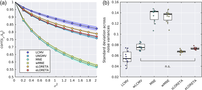
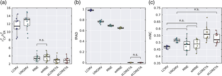
Noninvasive functional neuroimaging of the human brain can give crucial insight into the mechanisms that underpin healthy cognition and neurological disorders. Magnetoencephalography (MEG) measures extracranial magnetic fields originating from neuronal activity with high temporal resolution, but requires source reconstruction to make neuroanatomical inferences from these signals. Many source reconstruction algorithms are available, and have been widely evaluated in the context of localizing task-evoked activities. However, no consensus yet exists on the optimum algorithm for resting-state data. Here, we evaluated the performance of six commonly-used source reconstruction algorithms based on minimum-norm and beamforming estimates. Using human resting-state MEG, we compared the algorithms using quantitative metrics, including resolution properties of inverse solutions and explained variance in sensor-level data. Next, we proposed a data-driven approach to reduce the atlas from the Human Connectome Project's multi-modal parcellation of the human cortex based on metrics such as MEG signal-to-noise-ratio and resting-state functional connectivity gradients. This procedure produced a reduced cortical atlas with 230 regions, optimized to match the spatial resolution and the rank of MEG data from the current generation of MEG scanners. Our results show that there is no "one size fits all" algorithm, and make recommendations on the appropriate algorithms depending on the data and aimed analyses. Our comprehensive comparisons and recommendations can serve as a guide for choosing appropriate methodologies in future studies of resting-state MEG.

Keywords: Magnetoencephalography; cortical atlas parcellation; resolution analysis; resting-state; source reconstruction.

FIGURE 1

Variance explained analysis methods of comparing source reconstruction algorithms. (a) Variance explained analysis. Two hundred seventy‐four channel MEG data are split into 27 partitions of 10–11 sensors. For each cross‐validation fold, one partition is used as a test data set and all other folds are used as training data. For each algorithm, the training data are source reconstructed to gain an estimate of source dynamics. This source‐reconstructed activity is then forward mapped to the left out test sensors, and the temporal variance of the data recorded at these sensors explained by the brain activity is calculated as squared (temporal) correlation. The $r_{\mathit{CV}}^2$ measure reported here is the average variance explained at each test sensor, averaged over folds. For visualization, we demonstrate a single test sensor. The same methods are repeated for empty‐room recordings, and we use ratio of variance explained in resting‐state versus empty room recordings as our measure of interest. (b,c) Resolution analysis. (b) For a seed voxel, the corresponding column of the resolution matrix (the point spread function; PSF) relates unit “true” activity at that voxel to source estimates at each voxel. The distance between the seed voxel and the voxel at the peak of the PSF is the PAD. Shown is an example PSF for a seed voxel at the red diamond. The arrow points from the seed to the peak of the PSF, and the length of the arrow is PAD. The SEPS is the PSF‐weighted sum of distances to each voxel from the seed. (c) Rows of the resolution matrix (the cross talk function; CTF) quantifies the influence of “true” activity at all voxels on the source estimate of the seed voxel. The SECT is the CTF analogue of SEPS. Here we show an example CTF for a seed voxel at the red diamond. In b,c, figures are plotted on the smoothed cortical surface for visualization purposes only. (d) External noise analysis. To test robustness to external noise, white noise is added to the MEG sensor‐level data. Correlation between source‐space solutions with and without added sensor noise is computed. The level of reduction in correlation as the sensor‐level noise increased quantifies an algorithm's sensitivity to external noise

FIGURE 2

Correlation between different source reconstruction algorithms. Each algorithm was used to source reconstruct the MEG data, and correlation in the source space solutions of each pair of algorithms was calculated. For each pair of algorithms, the background color of the correlation matrix represents median value of correlation over all participants, while the inlaid plot shows the distribution over all subjects (the x‐axis is calibrated evenly for all plots, in the range [0,1]). No negative correlations were found. Hierarchical clustering of the median network is shown on the right to group algorithms based on similarity. Clustering used a spectral normalized cuts algorithm (Shi & Malik, 2000), and the x‐axis shows the cost of the cut. Therefore clusters with higher cost‐of‐cut are more strongly clustered, that is, contain higher correlations between algorithms

FIGURE 3

Statistics from variance explained and resolution analysis. (a) Ratio of cross‐validated variance explained in empirical data and empty room recordings ($r_{\mathit{CV}}^2/r_{\mathit{ER}}^2$) for each source reconstruction algorithm. (b) Peak activity displacement (PAD). (c) Spatial extent of cross talk (SECT). (d) Spatial extent of point spread (SEPS). For all figures, group‐wise analyses demonstrated a significant effect of algorithms. Pairwise analyses identified significant differences for all pairs except those marked as nonsignificant (n.s.), following false discovery rate correction. In the box plots, the range (whiskers), interquartile range (boxes), median (horizontal line), are shown, with values for each participant marked by dots to the left

FIGURE 4

Spatial distributions of resolution metrics. (a–c) Lateral and medial views (left and right columns) of PAD, SECT, and SEPS (respectively) for each dipole in each algorithm. (d) The norm of the leadfield for each dipole. (e) Anatomical maps of gyri and sulci, derived in Freesurfer. For all figures, distributions are shown on a smoothed cortical surface for visualization purposes, and are shown for the same representative participant

FIGURE 5

Correlation between source space solutions as sensor noise is added. Noise was added to the sensor data with variance ${\sigma }^2\cdot \text{trace}\left(C_x\right)/N_x$, where $C_x$ is the sensor data covariance matrix and $N_x$ is the number of sensors. We denote $s_{\sigma }$ as the source space solution to the noisy sensor data (without cross‐validation). The regularization parameter was adjusted according to the new predicted SNR due to added noise. (a) Correlation (averaged over dipoles) between $s_{\sigma }$ and $s_0$ (i.e., the source‐spaced solutions with and without noise added respectively) against noise variance ${\sigma }^2$. Shaded areas shown standard error of the mean. (b) The standard deviation of $\text{corr}\left(s_{\sigma },s_0\right)$ across noise levels, which (due to the monotonic decrease in correlation scores as noise increases) quantifies the extent to which an algorithm's solution changes as noise is artificially added. There was a significant difference between all pairs of algorithms except those marked nonsignificant (n.s.)

FIGURE 6

The reduced HCP‐MMP atlas. (a–c) The original atlas (Glasser et al., 2016), consisting of 180 ROIs per hemisphere split into 22 larger “clusters.” (a) The norm of the leadfield, summed over all voxels in an ROI $\omega$ (as a percentage of the sum over all ROIs), quantifying the strength with which $\omega$ influences the MEG. Clusters are marked by different colors, while each bar is an individual ROI. (b) Each ROI's anatomical location, plotted on the inflated Freesurfer average brain. Top shows the lateral surface, while the bottom is angled to show the medial and ventral surfaces. (c) As in b, but plotting only ROIs, which are modified in the reduced atlas to highlight changes. (d–f) The reduced atlas, consisting of 115 ROIs per hemisphere, plotted similarly as in a–c, respectively. We reduce the atlas by stating that each cluster should have a number of ROIs proportional to its influence on the MEG (a,d). For example, cluster 12 (the insula, the pink cluster marked in a and d by a black bar) has very many weak ROIs, so we combine these ROIs into fewer, larger, more influential ROIs. The result of this is a more uniform distribution of ROI strengths. While the calculation of numbers of ROIs per cluster was automated, the choice of which specific ROIs to be combined was made by hand from studying anatomical and functional closeness, based on the study of Glasser et al. (2016)

FIGURE 7

Parcellation based statistics. (a) Ratio of cross‐validated variance explained in empirical data and empty room recordings ($r_{\mathit{CV}}^2/r_{\mathit{ER}}^2$) for parcellated data. (b) Fractional peak activity displacement (fPAD). (c) Mean neighbor correlation (mNC) of ROI time series. For all figures, group‐wise analyses demonstrated a significant effect of algorithms. In these figures, pairwise analyses identified significant differences for all pairs except those marked as nonsignificant (n.s.), following false discovery rate correction. The meaning of whiskers, boxes, and so on are explained in Figure 3

References

1. Anzolin, A., Presti, P., Van De Steen, D., Astolfi, L., Haufe, S., & Marinazzo, D. (2019). Quantifying the effect of demixing approaches on directed connectivity estimated between reconstructed EEG sources. Brain Topography, 32(4), 655–674. 10.1007/s10548-019-00705-z - DOI - PubMed
1. Babiloni, C., Lizio, R., Marzano, N., Capotosto, P., Soricelli, A., Triggiani, A., … Del Percio, C. (2016). Brain neural synchronization and functional coupling in Alzheimer's disease as revealed by resting state EEG rhythms. International Journal of Psychophysiology, 103, 88–102. 10.1016/j.ijpsycho.2015.02.008 - DOI - PubMed
1. Bai, X., Towle, V., He, E., & Bin, H. (2007). Evaluation of cortical current density imaging methods using intracranial electrocorticograms and functional MRI. NeuroImage, 35, 598–608. 10.1016/j.neuroimage.2006.12.026 - DOI - PMC - PubMed
1. Baker, A., Brookes, M., Smith, S., Behrens, T., Probert Smith, P., & Woolrich, M. (2014). Fast transient networks in spontaneous human brain activity. eLife, 3, e01867. 10.7554/eLife.01867 - DOI - PMC - PubMed
1. Barzegaran, E., & Knyazeva, M. (2017). Functional connectivity analysis in EEG source space: the choice of method. PLoS One, 12(7), e0181105. 10.1371/journal.pone.0181105 - DOI - PMC - PubMed
Publication types