Global distribution patterns of marine nitrogen-fixers by imaging and molecular methods

Abstract

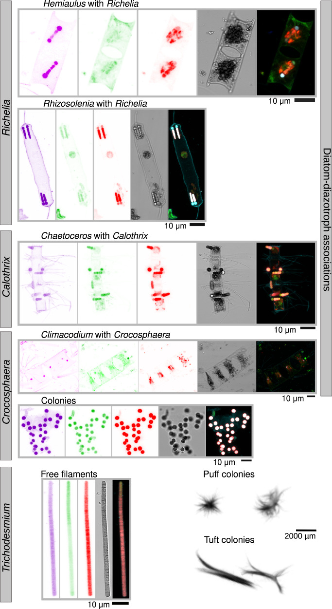
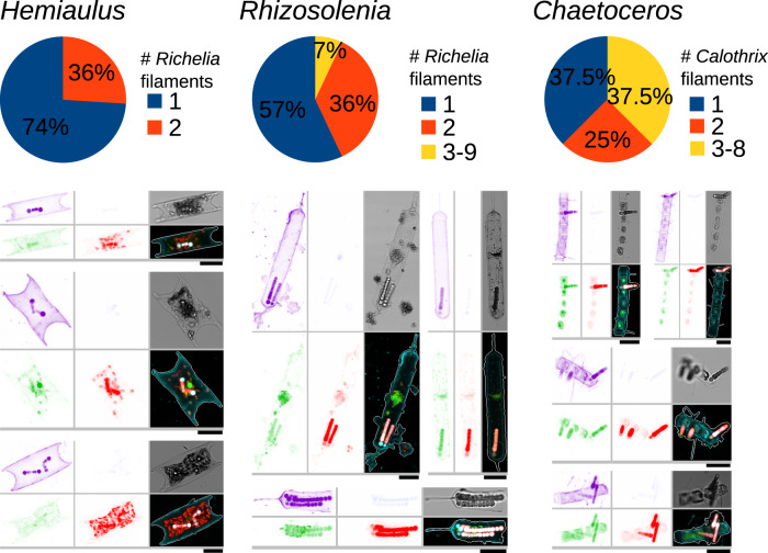
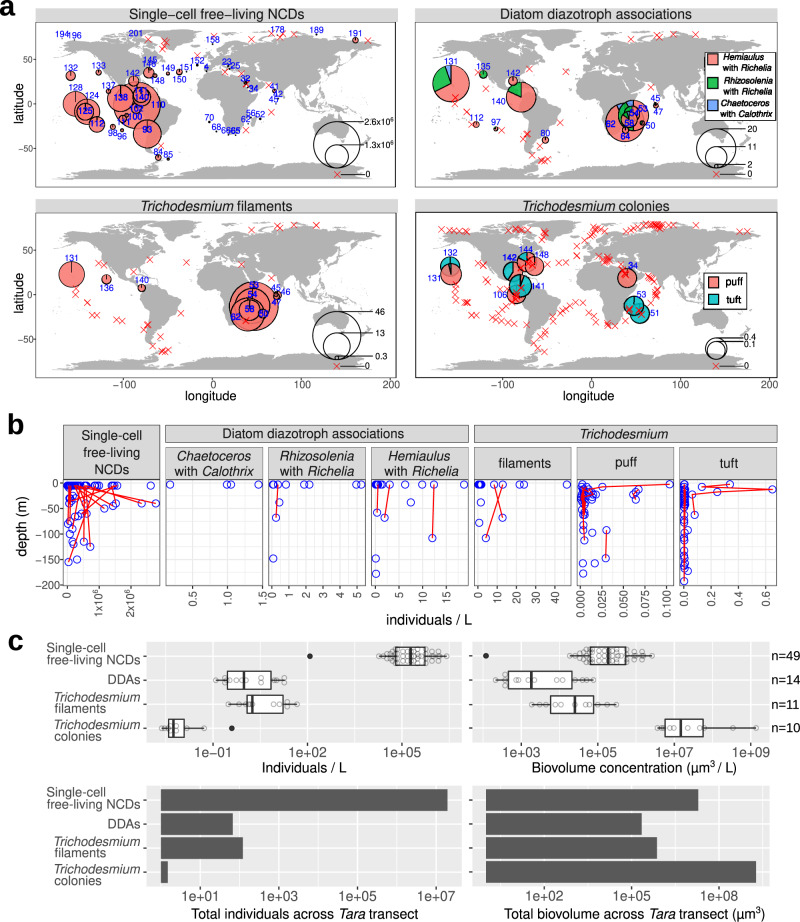
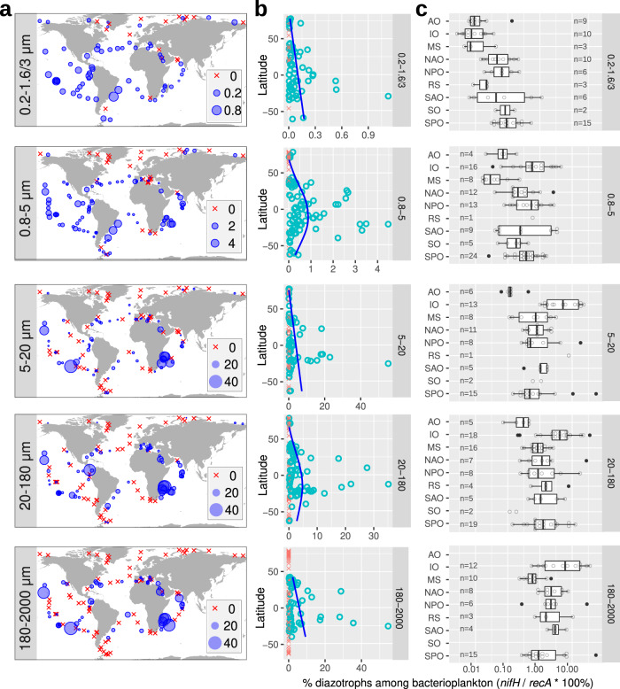
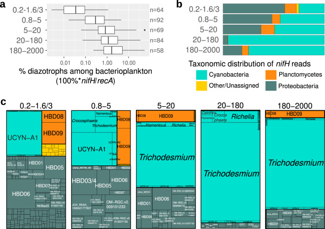
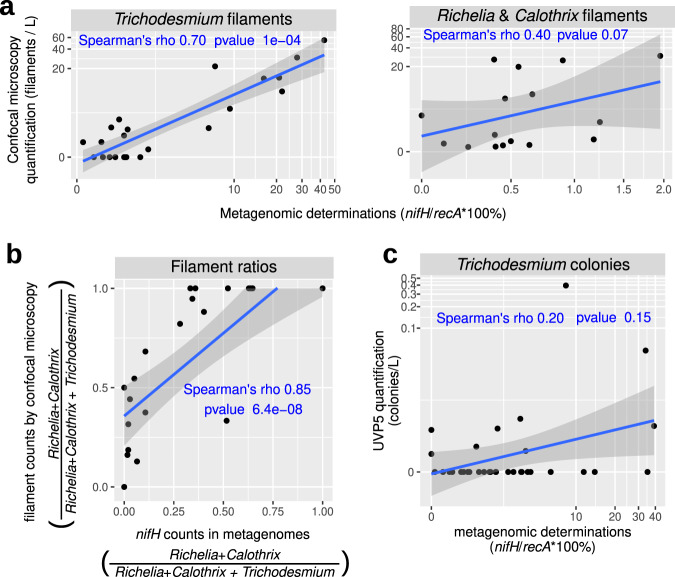
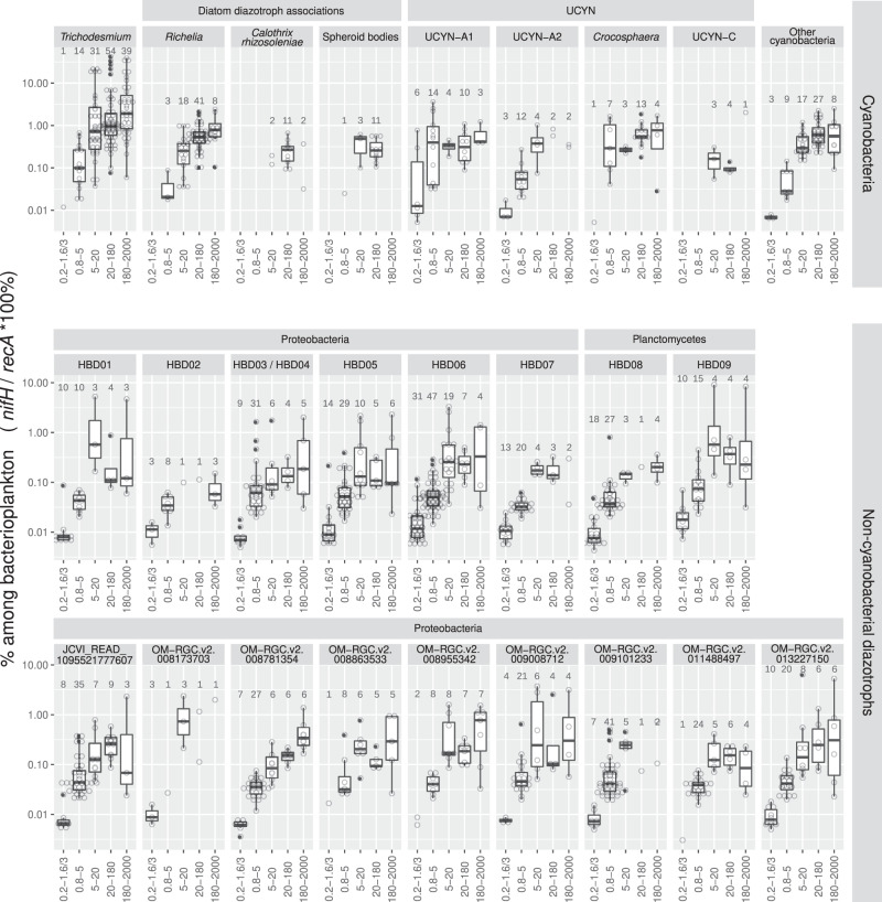
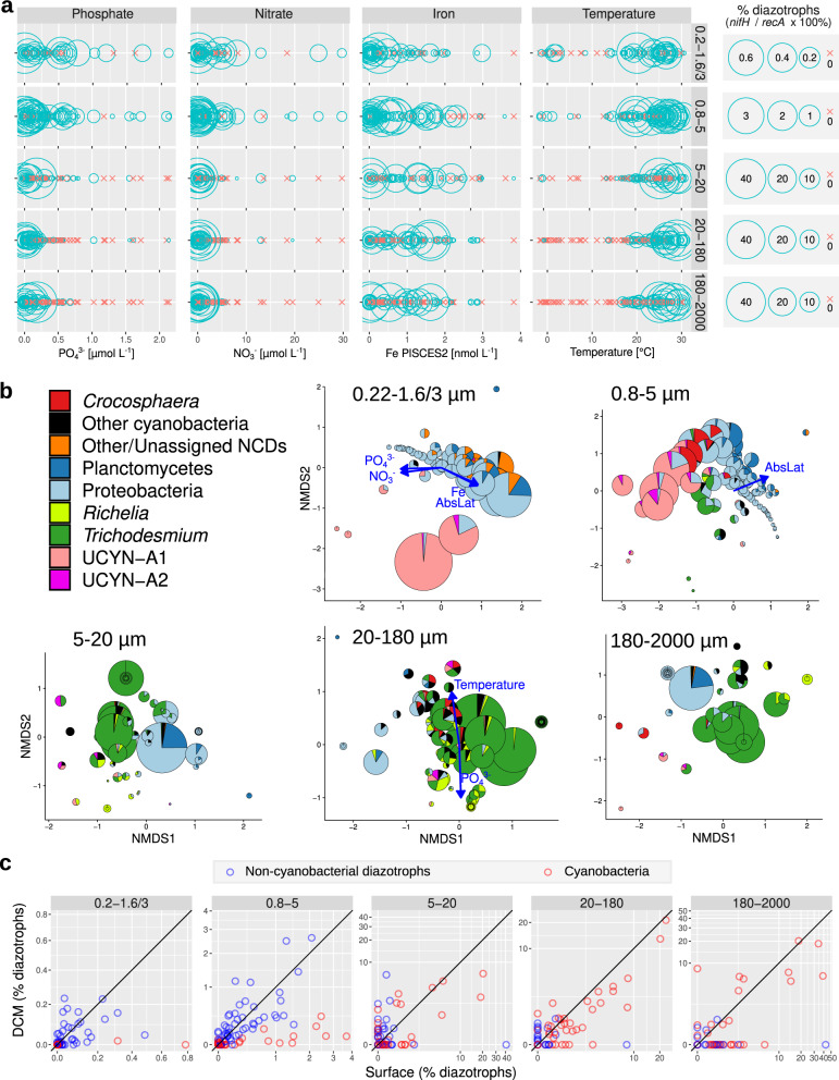
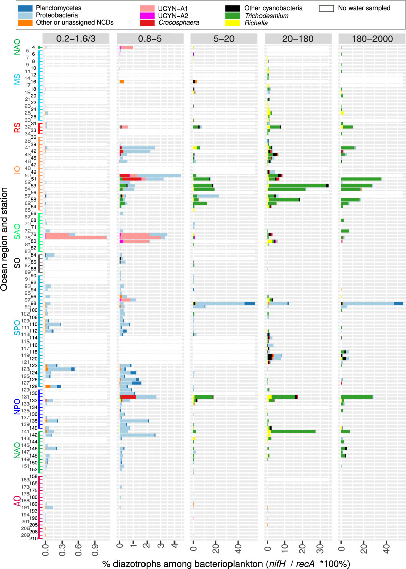
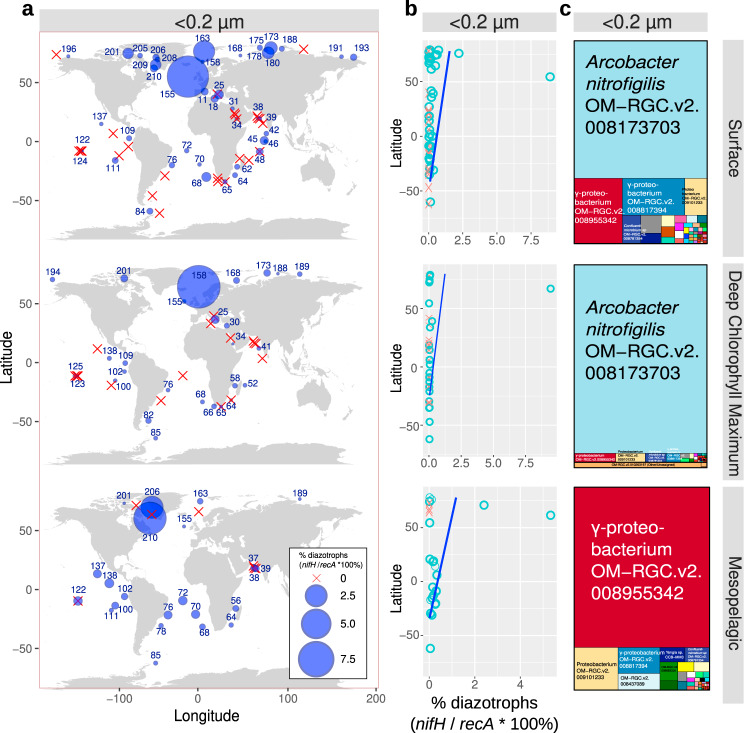
Nitrogen fixation has a critical role in marine primary production, yet our understanding of marine nitrogen-fixers (diazotrophs) is hindered by limited observations. Here, we report a quantitative image analysis pipeline combined with mapping of molecular markers for mining >2,000,000 images and >1300 metagenomes from surface, deep chlorophyll maximum and mesopelagic seawater samples across 6 size fractions (<0.2-2000 μm). We use this approach to characterise the diversity, abundance, biovolume and distribution of symbiotic, colony-forming and particle-associated diazotrophs at a global scale. We show that imaging and PCR-free molecular data are congruent. Sequence reads indicate diazotrophs are detected from the ultrasmall bacterioplankton (<0.2 μm) to mesoplankton (180-2000 μm) communities, while images predict numerous symbiotic and colony-forming diazotrophs (>20 µm). Using imaging and molecular data, we estimate that polyploidy can substantially affect gene abundances of symbiotic versus colony-forming diazotrophs. Our results support the canonical view that larger diazotrophs (>10 μm) dominate the tropical belts, while unicellular cyanobacterial and non-cyanobacterial diazotrophs are globally distributed in surface and mesopelagic layers. We describe co-occurring diazotrophic lineages of different lifestyles and identify high-density regions of diazotrophs in the global ocean. Overall, we provide an update of marine diazotroph biogeographical diversity and present a new bioimaging-bioinformatic workflow.

Fig. 1. Imaging observations of diazotrophs in Tara Oceans samples.

Images were obtained by environmental high content fluorescence microscopy (eHCFM; ref. ), with the exception of Trichodesmium colonies, which were detected in situ using an Underwater Vision Profiler 5 (UVP5; ref. ). From left to right, the displayed channels for each micrograph correspond to: cell surface (cyan, AlexaFluor 546), cellular membranes (green, DiOC6), chlorophyll autofluorescence (red), the bright field, and the merged channels. The displayed Hemiaulus-Richelia association was detected at station TARA_80 in the South Atlantic Ocean, Rhizosolenia-Richelia at TARA_53 in the Indian Ocean, Chaetoceros-Calothrix at TARA_131 (ALOHA) in the North Pacific Ocean, Climacodium-Croscophaera at TARA_140 in the North Pacific Ocean, the Croscophaera-like colony at TARA_53 in the Indian Ocean, the Trichodesmium filament at TARA_42 in the Indian Ocean, and the Trichodesmium colonies at TARA_141 and TARA_142 in the North Atlantic Ocean. Each micrograph is representative of the following number of images obtained in the current study: 350 Hemiaulus-Richelia, 56 Rhizosolenia-Richelia, 8 Chaetoceros-Calothrix, 1 Climacodium-Crocosphaera, 150 Crocosphaera-like colonies, 605 Trichodesmium-free filaments, 115 puff and 95 tuft colonies of Trichodesmium.

Fig. 2. Variation in the number of Richelia/Calothrix filaments among the diatom-diazotroph associations observed by high-throughput confocal microscopy.

Examples of images are shown. Clockwise from top-left, the displayed channels for each micrograph correspond to: cell surface (cyan, AlexaFluor 546 dye), DNA (blue, Hoechst dye), the bright field, cellular membranes (green, DiOC6 dye), chlorophyll autofluorescence (red), and the merged channels. The size bar at the bottom left of each microscopy image corresponds to 10 μm.

Fig. 3. Abundance and distribution of diazotrophs by quantitative imaging methods.

a Biogeography in surface waters. Bubble size varies according to the corresponding diazotroph concentration (individuals/L), while red crosses indicate their absence. Station labels with detection of diazotrophs are indicated in blue. b Depth partition. Samples from the same geographical site are connected by red lines. c Distribution of individual abundances and biomass in surface waters. Single-cell free-living non-cyanobacterial diazotrophs (NCDs) were quantified by merging flow cytometry counts with nifH/recA ratio from metagenomes from size fraction 0.22–1.6/3 μm and assuming an average cellular biovolume of 1 μm³ based on the cell dimensions reported in the literature for cultured NCDs^–. The detection and biovolume determinations of diatom-diazotroph associations (DDAs) and Trichodesmium-free filaments were carried out by high-throughput confocal microscopy in samples from the 20–180 μm size fraction. In the case of Trichodesmium colonies, it was determined using in situ images from the UVP5. Boxplots depict the 25–75% quantile range of the dataset without zeros (the corresponding biologically independent seawater samples are indicated in the plot), with the center line depicting the median (50% quantile); whiskers encompass data points within 1.5× the interquartile range. Source data are provided as a Source data file.

Fig. 4. Biogeography of diazotrophs in surface waters using metagenomes obtained from different size-fractionated samples.

The percentage of diazotrophs in the bacterioplankton community was estimated by the ratio of metagenomic read abundance between the marker genes nifH and recA. a Biogeography. The bubble size varies according to the percentage of diazotrophs, while red crosses indicate absence (i.e., no detection of nifH reads). b Latitudinal abundance gradient. The blue lines correspond to generalized additive model smoothings. c Ocean distribution. MS Mediterranean Sea, IO Indian Ocean, SAO South Atlantic Ocean, SO Southern Ocean, SPO South Pacific Ocean, NPO North Pacific Ocean, NAO North Atlantic Ocean, AO Arctic Ocean. Boxplots depict the 25–75% quantile range of the dataset without zeros (the corresponding biologically independent seawater samples are indicated in the plot), with the center line depicting the median (50% quantile); whiskers encompass data points within 1.5× the interquartile range. Source data are provided as a Source data file.

Fig. 5. Abundance of diazotrophs in surface waters using metagenomes obtained from different size-fractionated samples.

a Diazotroph abundance. The percentage of diazotrophs in the bacterioplankton community was estimated by the ratio of metagenomic read abundance between the marker genes nifH and recA. b Taxonomic distribution of the nifH reads. c Taxonomic distribution at deeper resolution. HBD01 to HBD09 (heterotrophic bacterial diazotrophs) corresponds to the metagenome-assembled genomes from <3-µm size fractions. Boxplots depict the 25–75% quantile range of the dataset without zeros (the corresponding biologically independent seawater samples are indicated in the plot), with the center line depicting the median (50% quantile); whiskers encompass data points within 1.5× the interquartile range. Source data are provided as a Source data file.

Fig. 6. Correlation analysis between diazotroph quantifications by imaging and molecular methods.

a, b Comparison between environmental high content fluorescence microscopy (eHCFM) and metagenomics. Calothrix, Richelia, and Trichodesmium in samples from size fraction 20–180 μm were measured by quantification of high-throughput confocal microscopy images (filaments L⁻¹) and by metagenomic counts (% of diazotrophs in the bacterioplankton community by the ratio between the marker genes nifH and recA). a Correlation of relative abundances in metagenomes and absolute abundances by confocal microscopy for the three taxa. b Correlation between the ratio of abundances between taxa. c Comparison between Underwater Vision Profiler 5 (UVP5) and metagenomics. Trichodesmium colonies were measured by UVP5 quantification (colonies L⁻¹) and by metagenomic counts in the 180–2000 µm size-fractionated samples. Spearman’s rho correlation coefficients and uncorrected one-side p-values are displayed in blue. Source data are provided as a Source data file.

Fig. 7. Distribution of the main diazotroph taxa across metagenomes obtained in different size-fractionated samples from surface waters.

For each taxon, the percentage in the bacterioplankton community is estimated by the ratio of metagenomic read abundance between the marker genes nifH and recA. The lineages grouped into ‘Other cyanobacteria’ are displayed in the Source data File. The ‘OM-RGC.v2’ prefix indicates the nifH sequences assembled from the metagenomes of <3-μm size fractions, while HBD01 to HBD09 (heterotrophic bacterial diazotrophs) corresponds to the metagenome-assembled genomes from the same samples. Boxplots depict the 25–75% quantile range of the dataset without zeros (the corresponding biologically independent seawater samples are indicated in the plot), with the center line depicting the median (50% quantile); whiskers encompass data points within 1.5× the interquartile range. Source data are provided as a Source data file.

Fig. 8. Environmental parameters and diazotroph distributions.

a Distribution across gradients of nutrients and temperature in surface waters. Blue circles correspond to samples with diazotrophs, while red crosses indicate absence (i.e., no detection of nifH reads). b NMDS analysis of stations according to Bray–Curtis distance between diazotroph communities of size-fractionated surface samples. Fitted statistically significant physico-chemical parameters are displayed (adjusted P value < 0.05). NMDS stress values: 0.07276045, 0.1122258, 0.1452893, 0.09693721, and 0.07969211. c Depth distribution. The scatter plots compare the diazotroph abundances between surface (5 m) and deep chlorophyll maximum (DCM; 17–180 m) for cyanobacteria (red points) and non-cyanobacterial diazotrophs (NCDs, blue points). Axes are in the same scale and the diagonal line corresponds to a 1:1 slope. Source data are provided as a Source data file.

Fig. 9. Diazotroph community based on metagenomes from size-fractionated surface samples.

The percentage of diazotrophs in the bacterioplankton community was estimated by the ratio of metagenomic read abundance between the marker genes nifH and recA. The bar color code shows the taxonomic annotation, while the absence of water sample is indicated by a white bar. The Y-axis shows the Tara Oceans stations and the ocean regions. MS Mediterranean Sea, IO Indian Ocean, SAO South Atlantic Ocean, SO Southern Ocean, SPO South Pacific Ocean, NPO North Pacific Ocean, NAO North Atlantic Ocean, AO Arctic Ocean. The equivalent figure showing the DCM water layer is shown in Fig. S2 (note the differences in scales between both figures, showing the higher relative abundance of diazotrophs in the surface layer). Source data are provided as a Source data file.

Fig. 10. Detection of ultrasmall diazotrophs in metagenomes obtained from <0.22 µm size-fractionated samples of different water layers.

The percentage of diazotrophs among ultrasmall bacterioplankton was estimated by the ratio of metagenomic read abundance between the marker genes nifH and recA. a Biogeography. The bubble size varies according to the percentage of diazotrophs, while red crosses indicate absence (i.e., no detection of nifH reads). Station labels with diazotrophs detection are indicated in blue. b Latitudinal abundance gradient. Circles correspond to samples with diazotrophs, while crosses indicate absence. The blue lines correspond to generalized additive model smoothings. c Taxonomic distribution of the nifH reads. The ‘OM-RGC.v2’ prefix indicates the nifH sequences assembled from metagenomes of <3 μm size fractions, including <0.22 μm. Source data are provided as a Source data file.

References

1. Field CB, Behrenfeld MJ, Randerson JT, Falkowski P. Primary production of the biosphere: integrating terrestrial and oceanic components. Science. 1998;281:237–240. doi: 10.1126/science.281.5374.237. - DOI - PubMed
1. Moore CM, et al. Processes and patterns of oceanic nutrient limitation. Nat. Geosci. 2013;6:701–710. doi: 10.1038/ngeo1765. - DOI
1. Tyrrell T. The relative influences of nitrogen and phosphorus on oceanic primary production. Nature. 1999;400:525–531. doi: 10.1038/22941. - DOI
1. Falkowski PG. Evolution of the nitrogen cycle and its influence on the biological sequestration of CO2 in the ocean. Nature. 1997;387:272–275. doi: 10.1038/387272a0. - DOI
1. Karl D, et al. The role of nitrogen fixation in biogeochemical cycling in the subtropical North Pacific Ocean. Nature. 1997;388:533–538. doi: 10.1038/41474. - DOI
Publication types