Engineering phase and polarization singularity sheets

Abstract

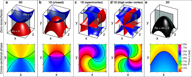
Optical phase singularities are zeros of a scalar light field. The most systematically studied class of singular fields is vortices: beams with helical wavefronts and a linear (1D) singularity along the optical axis. Beyond these common and stable 1D topologies, we show that a broader family of zero-dimensional (point) and two-dimensional (sheet) singularities can be engineered. We realize sheet singularities by maximizing the field phase gradient at the desired positions. These sheets, owning to their precise alignment requirements, would otherwise only be observed in rare scenarios with high symmetry. Furthermore, by applying an analogous procedure to the full vectorial electric field, we can engineer paraxial transverse polarization singularity sheets. As validation, we experimentally realize phase and polarization singularity sheets with heart-shaped cross-sections using metasurfaces. Singularity engineering of the dark enables new degrees of freedom for light-matter interaction and can inspire similar field topologies beyond optics, from electron beams to acoustics.

Fig. 1. Intersection topologies of zero-isosurfaces that form optical singularities.

Optical singularities are formed at the intersection of the zero-isosurfaces of the real (Re) and imaginary (Im) parts of a complex field (e.g., a linearly polarized electric field). Top row: intersection topologies of the two zero-isosurfaces (blue: Re = 0, red: Im = 0). Bottom row: phase profiles for each intersection topology in the top row, evaluated at the gray cross-sectional plane. Black lines indicate the zero-valued contours on the cross-sectional plane. a When the zero-isosurfaces intersect at a point, a 0D point singularity is formed. 1D singularities can be formed as b a closed loop or c, d an open line. c The fundamental Laguerre–Gaussian_0,1 vortex beam, with its corkscrew-like zero-isosurfaces. d A higher-order Laguerre–Gaussian_0,2 vortex beam has more than one pair of zero-sheets intersecting along a line. e When the zero-isosurfaces coincide, the singularity is 2D.

Fig. 2. Comparison between phase gradient maximization and field minimization to obtain phase singularities.

Both methods can be used to obtain phase singularities, but they produce different field behavior in terms of its real (blue) and imaginary (red) zero-isosurfaces. Yellow dots label the positions at which the field and phase gradients are optimized. Inset surface plots are the logarithmically scaled field intensities at z = 0 μm over the same XY domain. The z = 0 μm plane is indicated with the gray plane in each isosurface plot. a When the phase gradient in a specified direction is maximized, the two zero-isosurfaces align approximately tangentially and in the direction normal to that specified gradient. This produces a flat low field intensity structure along these aligned zero-isosurfaces. b Minimizing the field amplitude at a point to produce a singularity merely enforces a crossing of the zero-isosurfaces without any alignment, producing a 1D line singularity. c Simultaneously optimizing two nearby points with directed phase gradients can extend the range of the singularity sheet. d Minimizing the field amplitude at two points simultaneously does not guarantee alignment of the zero-isosurfaces and can instead produce multiple crossing lines, each producing a 1D line singularity.

Fig. 3. An engineered heart-shaped optical phase-singularity sheet (λ₀ = 532 nm).

a Isosurface of low field intensity for the simulated singularity sheet. The phase gradient was maximized in the directions indicated by the arrows on the gray z = 10 mm plane, at the locations of the yellow dots. b Inverse-designed phase profile, located at z = 0 mm, which realizes the heart-shaped optical singularity. c The 1D cut profile of intensity, phase, and phase gradient magnitude |∇_⊥ϕ| = [(∂_xϕ)² + (∂_yϕ)²]^1/2 for the dotted blue line in d, overlaid with the corresponding quantities for a Laguerre–Gaussian vortex beam. d Simulated relative intensity and g phase profile of the singularity sheet, at z = 10 mm. e Relative intensity profile obtained experimentally with a fabricated metasurface and h phase profile (obtained from iterative phase retrieval), at z = 10 mm. As a comparison, the results of Gerchberg–Saxton (GS) iterative optimization to get the same heart pattern on the z = 10 mm plane are plotted in f for the intensity and in i for the phase at the target plane, which demonstrates lower pattern fidelity and contrast as compared to the phase gradient maximization result.

Fig. 4. Fabrication and characterization of the heart-shaped phase-singularity sheet.

a Left, scanning electron micrograph of the fabricated metasurface. This metasurface comprises 101 × 101 superpixels with a pitch of 8 μm. Each superpixel comprises a uniform 32 × 32 array of cylindrical nanopillars with a pitch of 0.25 μm. a Right, high-magnification SEM of the interface between two superpixels. b Experimental setup for the optical characterization of the heart-shaped phase singularity. The ×100 objective (numerical aperture (NA) = 0.95) is scanned over 41 z-positions (from 9.6 to 10.4 mm) to capture the longitudinal variation of the phase singularity using a complementary metal oxide semiconductor (CMOS) camera sensor. c Iterative single-beam multiple-intensity reconstruction phase retrieval algorithm used to estimate the phase profile at each z-position. During one cycle, the forward propagation is performed from the first image (at z = 9.6 mm) to each image and backwards to the first image. This cycle is performed 50 times to yield the 41 phase profiles at each z-position.

Fig. 5. An engineered heart-shaped optical polarization singularity sheet (λ₀ = 532 nm) profiled at various transverse planes.

The columns are, from left to right, experimental polarization azimuth Ψ, simulated polarization azimuth Ψ, experimental ellipticity angle θ, simulated ellipticity angle θ, experimental intensity (s₀ Stokes parameter) profile, and simulated intensity profile. Black and white ellipses in the azimuth plots indicate the local polarization ellipses. Black ellipses indicate left-handed elliptical polarization and white ellipses indicate right-handed elliptical polarization. The experimental optical field was produced by a polarization-sensitive metasurface. The images are captured at different displacements z from the metasurface along the propagating direction. The diagonal fringes in the experimental plots are artifacts arising from light diffracting around an iris in the optical path.

Fig. 6. Fabrication and characterization of the heart-shaped polarization singularity metasurface.

a Left, SEM image of the fabricated metasurface, which comprises 51 × 51 superpixels with a pitch of 8.4 μm. Each superpixel comprises 20 × 20 nanofins with a pitch of 0.42 μm. a Right, high-magnification SEM image at the interface of four pixels showing the individual nanofins. b Experimental setup for optical characterization of the 2D polarization singularity metasurface. The incident laser light is polarized at 45°. The transmitted light is magnified through a ×100 objective (numerical aperture (NA) = 0.95) before passing through a quarterwave plate and a horizontal analyzer. An image of the optical field is captured by a complementary metal oxide semiconductor (CMOS) camera sensor for every 5° of rotation of the quarterwave plate up to a total rotation angle of 180° from the horizontal. These images are used to reconstruct the polarization state of the optical field at a pixel-by-pixel level.

References

1. Nye JF, Berry M. Dislocations in wave trains. Proc. R. Soc. A Math. Phys. Eng. Sci. 1974;336:165–190.
1. Berry M. Making waves in physics. Nature. 2000;403:21. doi: 10.1038/47364. - DOI - PubMed
1. Dennis, M. R., O’Holleran, K. & Padgett, M. J. in Progress in Optics Ch. 5, 53 (Elsevier, 2009).
1. Ignatowsky, V. S. Diffraction by a lens of arbitrary aperture. Trans. Opt. Inst. Petr. 1, 1–36 (1919).
1. Richards B, Wolf E. Electromagnetic diffraction in optical systems, II. Structure of the image field in an aplanatic system. Proc. R Soc. Lond. Ser. A Math. Phys. Sci. 1959;253:358–379.