. 2021 Jul;595(7868):549-553.
doi: 10.1038/s41586-021-03714-w. Epub 2021 Jul 7.

Sexual arousal gates visual processing during Drosophila courtship

Affiliations

Sexual arousal gates visual processing during Drosophila courtship

Tom Hindmarsh Sten et al. Nature. 2021 Jul.

Abstract

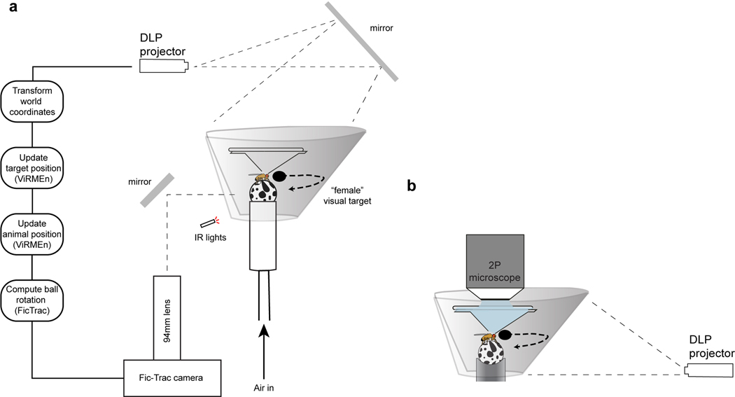
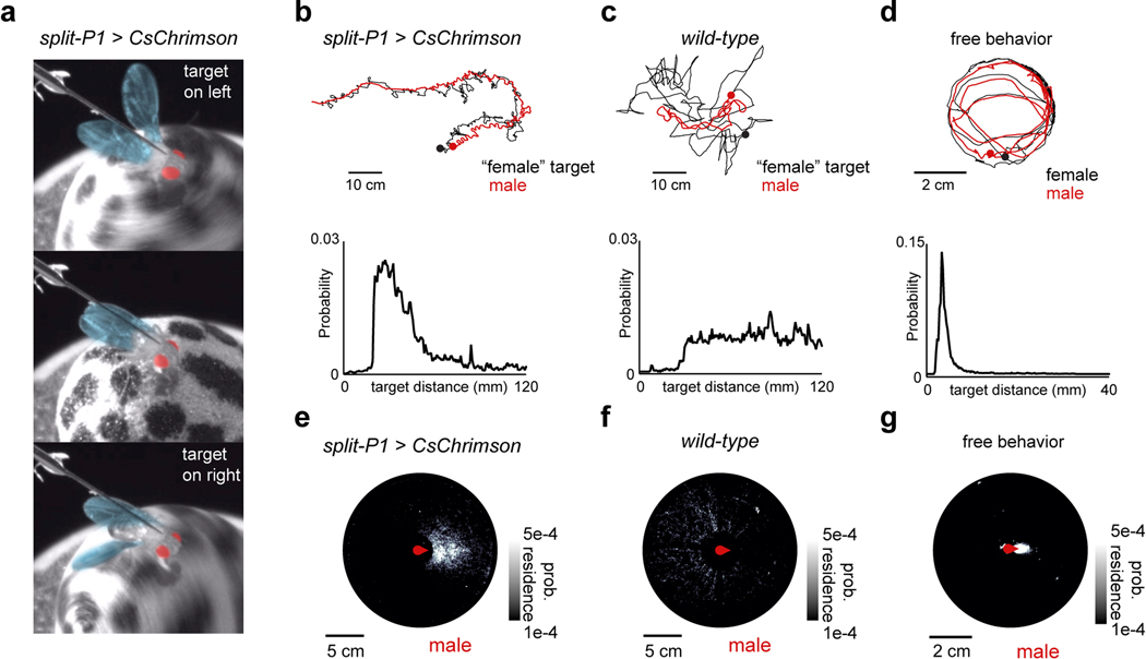
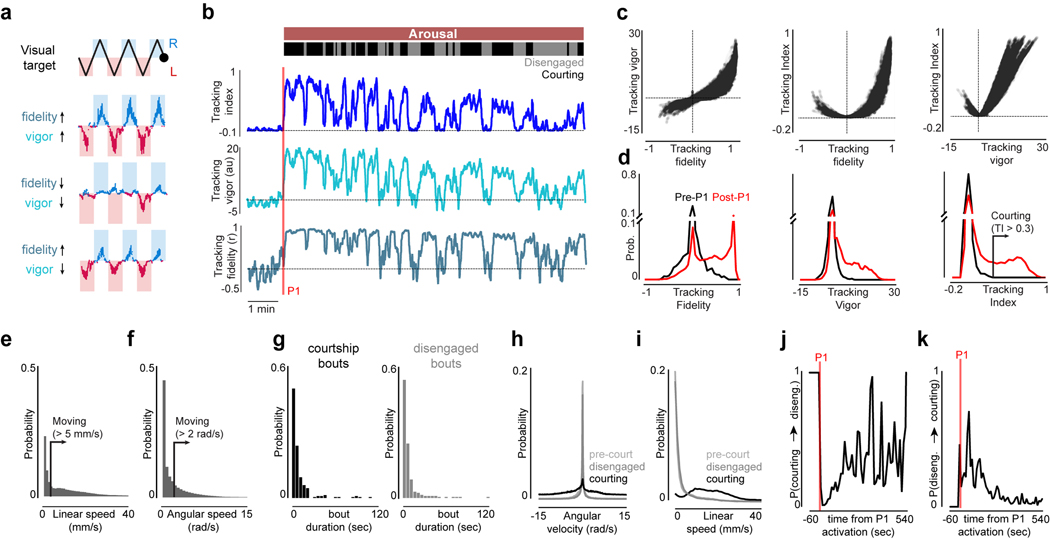
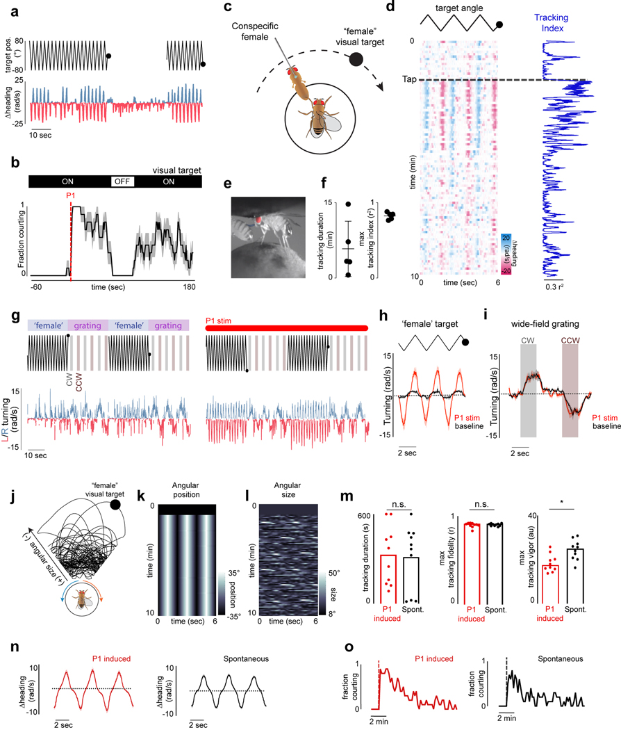
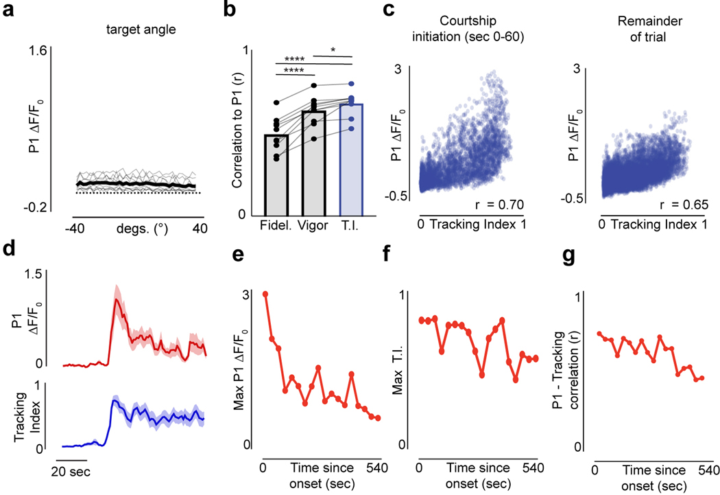
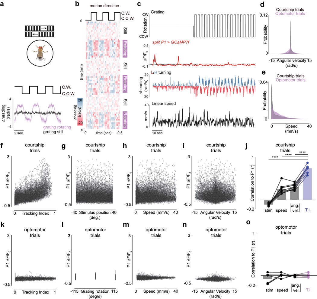
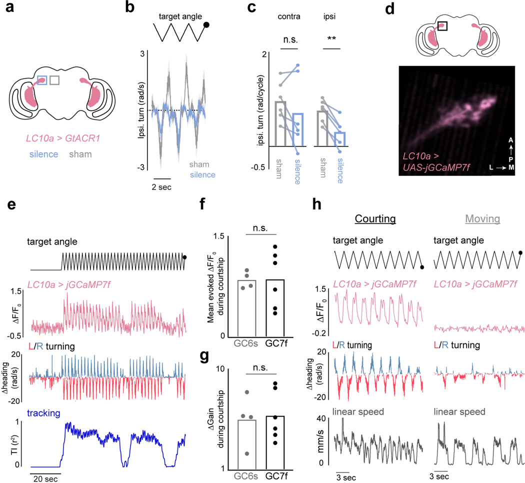
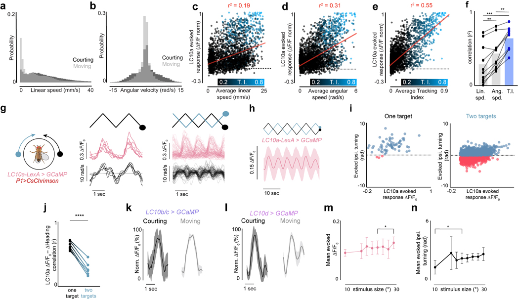
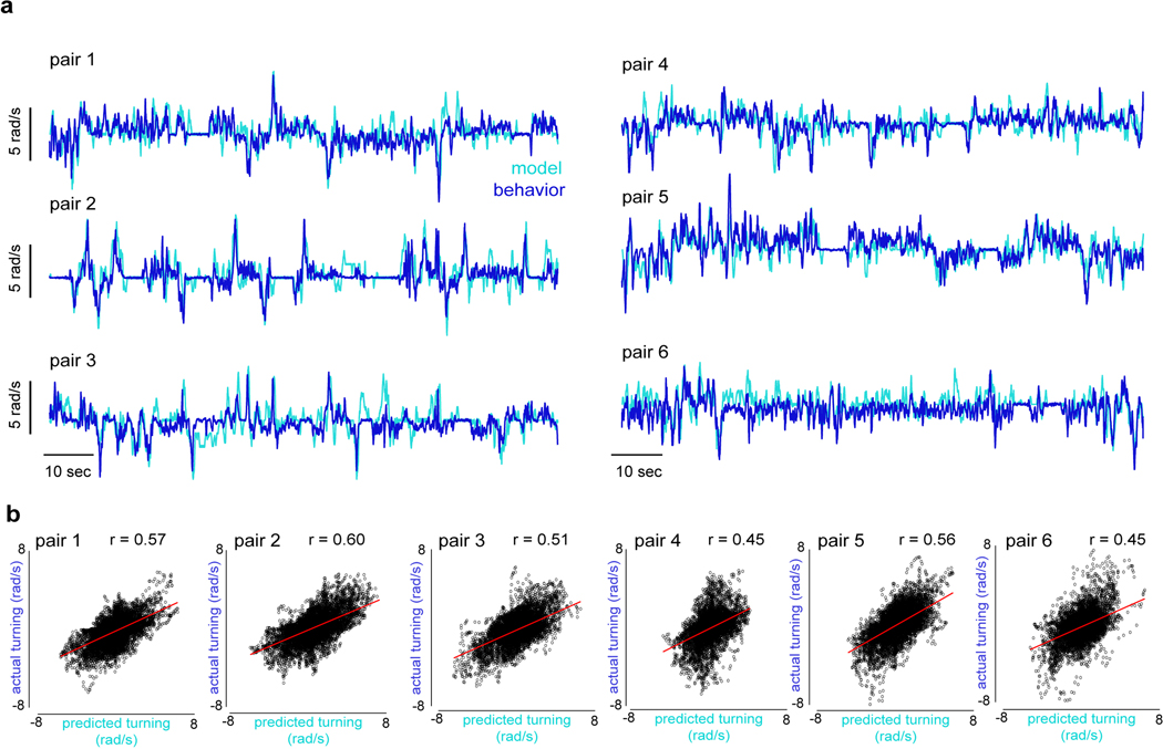
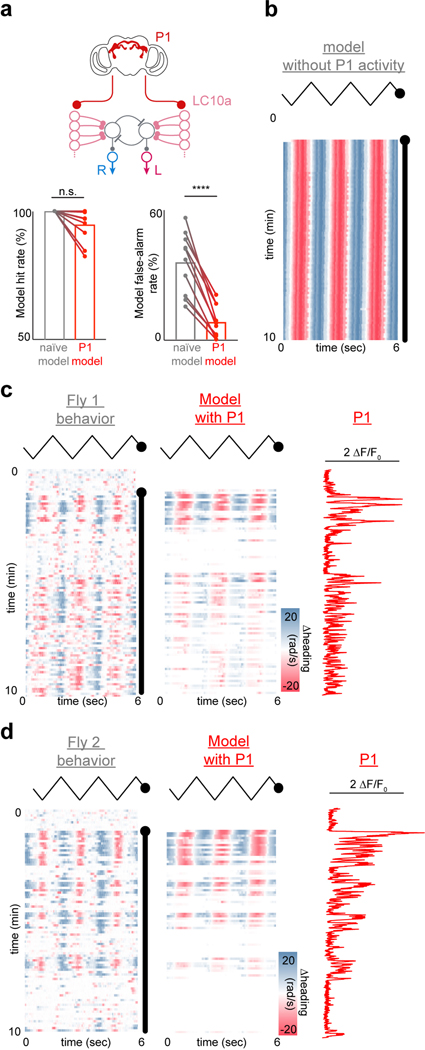
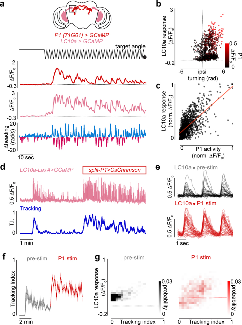
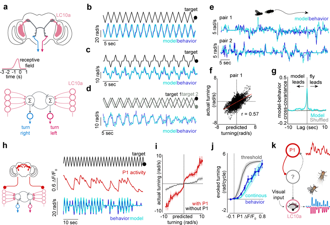
Long-lasting internal arousal states motivate and pattern ongoing behaviour, enabling the temporary emergence of innate behavioural programs that serve the needs of an animal, such as fighting, feeding, and mating. However, how internal states shape sensory processing or behaviour remains unclear. In Drosophila, male flies perform a lengthy and elaborate courtship ritual that is triggered by the activation of sexually dimorphic P1 neurons1-5, during which they faithfully follow and sing to a female6,7. Here, by recording from males as they court a virtual 'female', we gain insight into how the salience of visual cues is transformed by a male's internal arousal state to give rise to persistent courtship pursuit. The gain of LC10a visual projection neurons is selectively increased during courtship, enhancing their sensitivity to moving targets. A concise network model indicates that visual signalling through the LC10a circuit, once amplified by P1-mediated arousal, almost fully specifies a male's tracking of a female. Furthermore, P1 neuron activity correlates with ongoing fluctuations in the intensity of a male's pursuit to continuously tune the gain of the LC10a pathway. Together, these results reveal how a male's internal state can dynamically modulate the propagation of visual signals through a high-fidelity visuomotor circuit to guide his moment-to-moment performance of courtship.


Figures

Extended Data Figure 1 |
Extended Data Figure 1 |. A virtual reality preparation for tethered courtship.
a, Schematic of virtual reality preparation. Tethered male flies are placed on an air-cushioned foam ball, whose rotational velocity along all three axes is read out by a single camera via the FicTrac software. During closed-loop experiments, the male position in the virtual world is updated based on these rotations, as is the position of the target stimulus on the screen. Changes in the 2-D world are mapped to a conical screen and projected by way of a mirror from above. Hardware design by Jazz Weisman and Gaby Maimon. b, Schematic of the stimulus presentation during two-photon imaging. Due to sterics of the objective, the stimulus is rear-project onto the screen instead of from above as in (a).
Extended Data Figure 2 |
Extended Data Figure 2 |. Tethered courtship in an open 2-D virtual world.
a, Pseudocolor images of a courting male fly during activation of P1 neurons when the visual target is on his left (top), on his right (bottom), or in front of him (middle) showing ipsilateral wing extensions characteristic of courtship song. b, Top: position of the male and virtual female in the 2-D world during P1 activation over the course of 200 seconds. Bottom: histogram of the distance between the male and female target in top panel during closed-loop courtship. Note that male is bounded from bringing the stimulus closer than ~10mm from his position in the virtual world. c, Same as (b) but for a wild-type male. The increased jitter in the ‘female’ trajectory results from the target frequently reaching the maximum distance from the male and subsequently approaching him in a straight path. d, Top: Representative example of the 2D positions of the male and female in a freely courting pair of animals. Bottom: histogram of the distance between the male and female fly. e, Density plot of the relative position of virtual females with respect to the courting male during P1 activation. f, Same as (e) but for a wild-type male. g, Density plot of the location of the female relative to the male in freely courting pairs of animals. Details of statistical analyses and sample sizes are given in Supplementary Table 1.
Extended Data Figure 3 |
Extended Data Figure 3 |. The behavior of aroused animals is varied.
a, Schematic illustrating the distinction between vigor and fidelity of a male’s courtship pursuit. Vigor is quantified as the total turning in the direction of the visual target (normalized within-animal), while fidelity is the correlation between the visual target and the male’s turning. b, Characteristic example of the vigor, fidelity, and tracking index over the course of a courtship trial. P1 activation is denoted by red line. The male is classified as courting when T.I. > 0.3, and as disengaged when T.I. < 0.3 but he remains primed to reinitiate courtship pursuit. c, Comparison between the tracking fidelity, tracking vigor, and tracking index across animals. Each dot represents one frame; black lines indicate zero on axis. d, Distribution of tracking fidelity, tracking vigor, and tracking index across animals, before (black) and after (red) brief activation of P1 neurons. TI>0.3 will be used as a cutoff for courtship. e-f, Distribution of linear speeds (e) and angular speeds (f) observed during courtship trials. Lines indicate the thresholds used for denoting animals as “moving” (e.g., Fig 3f–g). g, Distribution of the duration of bouts of courtship (black) and bouts of disengagement after transient P1 activation. h, Distributions of the angular velocity exhibited by animals that are actively courting (black), that are disengaged (dark gray), and animals watching the visual stimulus before P1 activation (light gray). i, same as (h) but for linear speeds. j, Probability that an animal that is currently courting will transition to disengagement in any given second, plotted over the course of a trial in 10-second bins (red line denotes P1 activation). k, Probability that an animal that is disengaged will transition to courtship in any given second, plotted over the course of a trial in 10-second bins (red line denotes P1 activation). Details of statistical analyses and sample sizes are given in Supplementary Table 1.
Extended Data Figure 4 |
Extended Data Figure 4 |. Acute and enduring regulation of courtship arousal.
a, Male orienting before, during, and after the visual target was transiently removed from the screen (30 s). Courtship arousal was induced by a 3-second optogenetic activation of P1 neurons expressing CsChrimson 60 seconds before stimulus removal. b, Average tracking index of males during stimulus-removal trials (mean±s.e.m.). P1 neurons were transiently activated 1 min after the visual target began to oscillate, and temporarily removed from the screen for 30 seconds one minute after P1 activation. c, Schematic of the preparation allowing male to sample gustatory pheromones to trigger courtship. The male fly is provided with the abdomen of a virgin female to taste with his foreleg while the visual target oscillates on the screen in front of him. d, Example of a male’s turning during a courtship trial, before and after the male tapped the female abdomen with his foreleg (black line indicates tap). Each row consists of three stimulus cycles. e, Pseudocolor image of a male fly sampling the pheromones on a female abdomen. f, Maximal tracking index (right) and duration between the first and last detected bout of courtship (left) during pheromone induced courtship trials. g, Characteristic example of male turning during interleaved presentations of either a female target (black line) or a wide-field grating oscillating in the clockwise (CW: gray) or counter-clockwise (CCW: burgundy) before (left) or during (right) optogenetic activation of P1 neurons. h, Average male turning in response to three cycles of the oscillating female target before (black) or during (red) activation of P1 neurons. i, Average male turning in response to the wide-field grating rotating in the clockwise (gray) or counter-clockwise (burgundy) direction before (black) or during (red) activation of P1 neurons. Note that in difference to responses to the ‘female’ target in (h), optomotor responses were not enhanced during P1 activation. j, 2-D path of the dynamic visual target used for inducing spontaneous courtship. k,l, Angular position (k) and angular size (l) of the dynamic visual target subtended on the male retina over the course of a 10 minute trial. m, Duration between the first and last detected bout of courtship for courtship induced by optogenetic activation of P1 neurons versus spontaneous courtship (left), and the maximum tracking fidelity (middle) and vigor (right) displayed by animals in the two conditions. n, Average turning response during courtship in trials where courtship was induced by activation of P1 neurons (left) or spontaneously initiated (right). o, Fraction of males actively engaged in courtship (TI > 0.3) over the course of a 10-minute trial in P1 induced trials (left) and spontaneously initiated trials (right). Dashed lines indicate LED onset (red) or the onset of visual motion (right). All shaded line plots are mean±s.e.m.; * indicates p<0.05, ns indicates p>0.05; details of statistical analyses and sample sizes are given in Supplementary Table 1.
Extended Data Figure 5 |
Extended Data Figure 5 |. P1 neurons are dynamic but strongly correlated to the intensity of courtship pursuit.
a, The average activity of P1 neurons (ΔF/F0) plotted versus the position of the ‘female’ visual target. Thin grey lines are individual animals, black line is the average across animals. b, Correlation between P1 activity (ΔF/F0) and the tracking fidelity, tracking vigor, and tracking index (T.I.) of males. Individual data points are individual animals. c, P1 activity (ΔF/F0) versus tracking index at the onset of courtship (first 60 seconds; left) and for the remainder of the trial (right). d, Top: Average response of P1 neurons aligned to the onset of courtship; bottom: average Tracking Index aligned to the onset of courtship. Note that P1 activity is disproportionally elevated in the first few seconds, indicating it may reflect additional aspects of the male’s internal state or behavior we are not measuring. e, Maximum P1 activity observed across animals as a function of time since courtship initiation. f, Maximum tracking index observed across animals as a function of time since courtship initiation. g, Average correlation between P1 activity (ΔF/F0) and the tracking index across animals as a function of time since courtship initiation. All shaded line plots are mean±s.e.m.; ****indicates p<0.0001, *indicates p<0.05; details of statistical analyses and sample sizes are given in Supplementary Table 1.
Extended Data Figure 6 |
Extended Data Figure 6 |. P1 neurons are uncorrelated from the motor implementation of courtship.
a, Schematic of preparation for evoking optomotor responses using wide-field motion (top), and the turning responses of animals presented with alternating-direction wide-field motion. b, Example of a male’s turning during an optomotor trial. Each row consists of three stimulus cycles. Purple bars indicate when the grating is rotating. c, Example of the functional response (ΔF/F0) of P1 neurons during an optomotor trial, before and during the grating oscillates, as well as the angular velocity and linear speed of the animal. d, Histogram of angular velocities observed during courtship trials (gray) and during optomotor trials (purple). e, Histogram of linear speeds observed during courtship trials (gray) and during optomotor trials (purple). f-i, Scatter plots of P1 activity versus the tracking index (f), the stimulus position (g), the linear speed (h) and the angular velocity (i) of all animals during courtship trials. j, Correlation between P1 activity and the parameters explored in k-n during courtship trials. Individual data points are animals. k-n, Scatter plots of P1 activity versus the optomotor tracking index (k), the velocity of the grating (l), the linear speed (m) and the angular velocity (n) of all animals during optomotor trials. o, Correlation between P1 activity and the parameters explored in p-s during optomotor trials. Individual data points are animals. All shaded line plots are mean±s.e.m.; *indicates p < 0.05, **indicates p < 0.01, *** indicates p < 0.001, and **** indicates p < 0.0001. Details of statistical analyses and group sizes are given in Supplementary Table 1.
Extended Data Figure 7 |
Extended Data Figure 7 |. LC10a signaling is necessary and amplified during courtship.
a, Schematic of LC10a neurons expressing GtACR1 with approximate ROIs used for silencing (or sham-silencing) in a single hemisphere. b, Average turning of one male to the visual stimulus during silencing of LC10a neurons in the right hemisphere versus sham trials. Note that male fails to execute turns in the direction ipsilateral to silencing. c, Average turning in the direction ipsilateral and contralateral to the hemisphere where LC10a was silenced, compared to sham trials. d, Image of LC10a axon terminals expressing jGCaMP7f in the anterior optic tubercle. e, Example of functional response (ΔF/F0) of LC10a neurons expressing jGCaMP7f during a courtship. Note that, in difference from recordings made using GCaMP6s (Fig. 2b), calcium transients return to baseline in-between responses with this faster indicator. e, Average evoked LC10a responses (ΔF/F0) to one stimulus cycle for animals expressing GCaMP6s versus jGCaMP7f. f, Average change in LC10a gain (distance between peak and through of evoked responses) for animals expressing GCaMP6s versus jGCaMP7f. g, Example of LC10a functional responses during courtship versus during a later period of undirected running with similar linear speed. All shaded line plots are mean±s.e.m.; n.s. indicates p > 0.05, and **indicates p < 0.01. Details of statistical analyses and group sizes are given in Supplementary Table 1.
Extended Data Figure 8 |
Extended Data Figure 8 |. LC10a gain can be dissociated from the motor implementation of courtship pursuit.
a-b, Histograms of the linear speeds (a) and angular velocities (b) exhibited by animals in periods classified as courtship versus periods classified as ‘moving’. c, Average evoked LC10a activity (ΔF/F0) when the stimulus swept across the ipsilateral hemifield versus the average linear speed of animals in the same time period, color coded by the average tracking index during the sweep. Red line is the linear fit. d-e, same as (c) but plotted against the average angular speed (d) or average tracking index (e) exhibited by animals. f, Correlation between LC10a activity and the linear speed, angular speed, and tracking index exhibited by animals. Individual data points denote individual animals. g, Left: schematic of animal being presented with two identical ‘female’ targets, moving in opposition and thus yielding identical stimulation to both eyes. Middle: Example of LC10a functional responses versus the position of a single target (top) and animal turning responses (bottom). Right: Same as Middle, but when the animal was later in the trial presented with two opposing targets. P1 neurons were activated continuously. Note that LC10a neurons responded even when male failed to turn ipsilaterally when two-targets were present. h, Average LC10 activity during presentation of two opposing visual targets (top). i, Left: average evoked LC10 activity during ipsilateral sweeps of the visual target versus the total turning exhibited in the direction of the visual target during the same period. Right: average evoked LC10 activity during ipsilateral sweeps of either of the two visual targets versus the total turning exhibited in the direction of the visual target during the same period. j, Correlation between LC10a evoked responses and ipsilateral turning. Individual data points denote individual animals. k, Average peak-normalized responses (ΔF/F0) of LC10b/c neurons during courtship versus during locomotion. l, same as (k) but for LC10d neurons. m,n, Average evoked LC10a functional response (ΔF/F0, k) and average evoked ipsiversive turning (n) as a function of the average angular size of the visual target on each stimulus cycle. All shaded line plots are mean±s.e.m.; n.s. indicates p > 0.05, *indicates p < 0.05, **indicates p < 0.01, and *** indicates p < 0.001, Details of statistical analyses and group sizes are given in Supplementary Table 1.
Extended Data Figure 9 |
Extended Data Figure 9 |. LC10a neurons exhibit sparse and selective connectivity in the central brain.
a, Examples of identified LC10a, LC10b, LC10c, and LC10d neurons in the female hemi-brain connectome. b, Morphology of all identified LC10a-d neurons (n = 248). c, Correlation matrix of the outputs from all LC10 neurons, sorted by their assigned subtype. Note that individual subtypes have strongly correlated outputs that are largely distinct from the output patterns of other subtypes. d, t-SNE plot of the output connectivity matrix of all identified LC10 neurons, labeled based on the manually assigned subtype. The output connectivity naturally segregates LC10 neurons into four groups. e,f, Same as (c-d), but based on the input connections to LC10 neurons. g, Morphology of all non-optical output neurons from LC10a neurons with at least 10 synaptic connections, grouped based on projections to the LALs (left) versus to the IB (right). h, same as (g), but for non-optical input neurons to LC10a neurons. i, Representative example of trans-synaptic tracing of LC10a neurons in the male using Trans-Tango. Magenta denotes labeled LC10a neurons, and cyan the labeled post-synaptic partners. Similar results were obtained across 4 male brains. j, Histogram of synaptic weights between all LC10a neurons and their post-synaptic partners. k, Number of input and output synapses to/from LC10a neurons from the 10 most common brain regions (Superior Intermediate Protocerebrum (SIP), Lateral Accessory Lobe (LAL), Superior Medial Protocerebrum (SMP), Inferior Bridge (IB), Superior Posterior Slope (SPS), Posterior Ventrolateral Protocerebrum (PVLP), Posteriolateral Protocerebrum (PLP), Superior Medial Protocerebrum (SMP), Wedge (WED),), (R/L) indicates the right and left hemisphere, respectively.
Extended Data Figure 10 |
Extended Data Figure 10 |. P1 neurons enhance the gain of LC10a neurons without altering their receptive fields.
a, Left: schematic of synchronous recordings from P1 neurons in the LPC and LC10a neurons in the AOTu. Middle: cross-covariance of P1 neuron activity and LC10a activity during spontaneous courtship trial. Right: same as middle, but zoomed in to highlight that P1 neurons activity leads LC10a activity. Maximum covariance occurred at lag = −500ms. b, LC10a responses to presentation of a 10° sweeping dot in the progressive or regressive direction before and during activation of P1 neurons. Top: Average LC10a response during presentation of a regressively (orange) or progressively (blue) moving stimulus in the absence of P1 activation; bottom: average LC10a response during presentation of a regressively (orange) or progressively (blue) moving stimulus in the presence of P1 activation. c-e, same as b but for a sweeping 25° sphere, a sweeping 10° wide tall bar, or an approaching sphere expanding from 10° at 20°/s. Red indicates P1stimulation and black indicates pre-stimulation baseline throughout. f, Response Modulation Index (see Methods) for each stimulus presented before and during P1 activation, indicating that responses to the distinct visual stimuli are near uniformly enhanced. g, Average evoked ipsilateral turning in response to progressive motion of the different targets during P1 activation, plotted versus the average evoked LC10 response in the same period. Note that turning responses evoked by the motion of these diverse stimuli were proportional to the magnitude of LC10a evoked calcium transients: sweeping dots evoked the strongest turns, bars evoked much weaker turns, and slowly looming spheres did not elicit any turning on average, presumably because both eyes are stimulated equally. h, Average evoked linear speed in response to progressive motion of the different targets during P1 activation, plotted versus the average evoked LC10 response in the same period. i, Direction Selectivity Index (see Methods) for sweeping stimuli presented during baseline recordings or during continuous P1 activation. Positive values indicate a preference for progressive motion, negative values indicate preference for regressive motion. All shaded line plots are mean±s.e.m.; n.s. indicates p>0.05; details of statistical analyses and sample sizes are given in Supplementary Table 1.
Extended Data Figure 11 |
Extended Data Figure 11 |. Motion-direction selectivity during courtship pursuit.
a, Left: example image of LC10a-LexA axon terminals in the AOTu, with 48 ROIs of strongly correlated pixels automatically selected using the CaImAn-CNMF framework overlayed. Right: same as left, but ROIs have been color-coded according to their exhibited direction selectivity index (positive values indicate a preference for progressive motion, negative values indicate preference for regressive motion). b, Heat map of the average evoked responses to progressive (right) and regressive (left) sweeps of the 25° sphere during P1 activation for the 48 ROIs shown in (a). Each row represents the average evoked fluorescence across 10 trials for each ROI. c, Average evoked responses to a progressive versus regressively moving 25° dot across all ROIs from all animals (300 ROIs across 7 males). d, Direction Selectivity Index for all ROIs across animals (see methods for details). Black line denotes zero; positive values indicate a selectivity for progressive motion, negative values indicate a selectivity for regressive motion. e, Top: schematic of monocular stimulation. ‘Female’ targets were presented to one eye alone, and moved in either the regressive or progressive direction with respect to that eye with a 5-sec ISI. Bottom: Average turning of males in response to monocular stimuli moving regressively (left) or progressive (right). f, Turning responses of LC10a circuit model without motion-direction selectivity, with regressive-motion selectivity, and with progressive-motion selectivity. g, Left: normalized LC10a receptive fields with varying rise-times (κ, see methods). Right: correlation between predicted and actual responses to the simple stimulus in b for the receptive fields shown to the left. h, From left: average turning response to a single stimulus cycle; predicted response from full model to a single stimulus cycle; predicted response of a model with no binocular overlap; predicted response of a model not selective for progressive versus regressive motion. i, Example of predicted versus actual turning response to two targets with a drifting phase-offset (as in Figure 5d) across the courtship trial. Black line indicates when first target is present, grey line indicates when the second target is present. j, Left: Average correlation between the Stim 1 and predicted turning (cyan) during dual dot presentations. Right: Average correlation between the Stim 1 and the turning of males during dual dot presentations. In gray is what the correlation to Stim 1 would be if the animal perfectly tracked the Stim 2. Positive x-values indicate that the first stimulus leads in phase. All shaded line plots are mean±s.e.m.; ** indicates p<0.01; **** indicates p<0.0001; details of statistical analyses and sample sizes are given in Supplementary Table 1.
Extended Data Figure 12 |
Extended Data Figure 12 |. Network model predicts turning dynamics of freely courting males.
a, Examples of predicted versus actual turning of freely courting males over the first 100 seconds of courtship. b, Frame-by-frame predicted versus actual male turning over the course of the full courtship trials for the pairs shown in a (5–10 minutes), red line denotes the linear fit. Details of statistical analyses and sample sizes are given in Supplementary Table 1.
Extended Data Figure 13 |
Extended Data Figure 13 |. Incorporating P1 neural activity improves model performance.
a, Hit rate (fraction of predicted turns accompanied by a real turn; true positive rate) and false-alarm rate (fraction of predicted turns not accompanied by a real turn; false positive rate) of the naïve model versus when input current to LC10a neurons is scaled by the functional responses of P1 neurons. b, Example of the predicted turning over a courtship trial by a “naïve-model” (as in Fig. 5a) in which input current to LC10a neurons is consistently high. c-d, Two examples of actual (left) versus predicted (middle) turning responses when the activity of P1 neurons (right) is incorporated into the model. Compare to naïve model in (g). Black lines indicate when stimulus is oscillating. Details of statistical analyses and sample sizes are given in Supplementary Table 1.
Figure 1 |
Figure 1 |. P1 neurons release and reflect a dynamic state of sexual arousal.
a, Schematic of behavioral setup. b, 2-D path of a male courting a pseudo-randomly moving target in closed-loop. c, Angular position of the target relative to males expressing CsChrimson in P1 neurons or wild-type animals during tethered closed-loop courtship. d, Example of a courting male displaying turning (middle) and wing-extensions (bottom) to the visual target in open-loop. e, Example of a male’s turning throughout a courtship trial. Each row consists of three stimulus cycles, with the target angle shown at top. Red line indicates 3-second P1 activation; black bar indicates when the visual stimulus is oscillating. f, Tracking Index (see Methods) for 10 flies following optogenetic activation of P1 neurons. Top trace is the same animal as in (e). g-h, Same as e-f but for spontaneously initiated courtship trials. i, Schematic of P1 neurons in the male brain. j, Example of P1 neuron activity (ΔF/F0) and Tracking Index of a male during a courtship trial. k, Zoomed-in view of the onset of courtship in (j). l, Activity of P1 neurons (average ΔF/F0) versus Tracking Index. m, Distribution of P1 activity (ΔF/F0) before courtship was initiated, during periods when males were temporarily disengaged, and during active courtship pursuit (Tracking Index > 0.3). n,o Activity of P1 neurons (average ΔF/F0) versus the male’s linear speed (n) or angular velocity (n). Shaded line plots are mean±s.e.m.; thin lines denote individual animals; n.s. indicates p > 0.05; **** indicates p <0.0001. Details of statistical analyses and sample sizes are given in Supplementary Table 1.
Figure 2 |
Figure 2 |. Modulation of LC10a neurons during courtship.
a, Schematic of LC10a neurons expressing GCaMP. b, Example of LC10a responses during a courtship trial. Angular position of the target (top row); activity (ΔF/F0) of LC10a neurons (middle); angular velocity of male (bottom). c, Schematic depicting different LC10 subtypes that innervate the AOTu. d, Responses of LC10a, LC10b/c, and LC10d neurons (average ΔF/F0) to the visual target during periods of courtship (left) or general locomotion (right). e, Responses (average ΔF/F0) of LC10a neurons normalized to peak activity during courtship and general locomotion. f, Activity (average ΔF/F0) of LC10a, LC10b/c, and LC10d neurons versus a male’s ipsiversive turning velocity. g, Sample 2D paths of two males before (black) and during optogenetic activation of LC10a neurons in the left (red) or right (blue) hemisphere. h, Average evoked ipsilateral turning during unilateral stimulation of LC10a neurons expressing CsChrimson. Shaded line plots are mean±s.e.m.; Details of statistical analyses and sample sizes are given in Supplementary Table 1.
Figure 3 |
Figure 3 |. P1 neurons represent intensity of courtship and acutely regulate pursuit.
a, Example of simultaneously imaged LC10a and P1 neuron activity, both expressing GCaMP; angular position of the target (top); functional responses (ΔF/F0) of P1 neurons (upper-middle row) and LC10a (lower-middle row) and angular velocity of male (bottom). b, LC10 activity (ΔF/F0) evoked by a single stimulus sweep versus the ipsiversive turning response of the male, color coded by the average P1 activity in the same time-period. c, Normalized LC10a responses to each stimulus sweep versus normalized average P1 activity in the same time period (r = 0.68, p<0.00001, m = 0.85, b=0.10). d, Example of Tracking Index and the activity of LC10a neurons in a male before and during optogenetic activation of P1 neurons expressing CsChrimson. e, Responses (ΔF/F0) of LC10a neurons during spontaneous courtship (top) and P1 activation (bottom) for the male in (d). f, Average Tracking Index across animals over the trials structured as in (d). g, Density plot of Tracking Index versus activity (ΔF/F0) of LC10a neurons on each stimulus cycle before (left) and during P1 activation (right) across males. Shaded line plots are mean±s.e.m. Details of statistical analyses and sample sizes are given in Supplementary Table 1.
Figure 4 |
Figure 4 |. A network model of LC10a neurons recapitulates male pursuit.
a, Proposed anatomy of the LC10a circuit with LAL neurons (grey) and descending neurons (blue/red) (top), LC10a temporal receptive fields (middle), and network model (bottom). b-d, Predicted versus actual turning of aroused males to (b) a single target, (c) to a single target that pauses for 500ms in front of the male, and (d) to two targets oscillating at different frequencies. e, Examples of predicted versus actual turning of males during free courtship. f, Predicted versus actual turning velocity across a free courtship trial (pair 1; r = 0.56). g, Average normalized cross-covariance between predicted and actual turning during free courtship vs. shuffled controls. h, Schematic of network model incorporating P1 activity (left), and example of actual versus predicted turning when P1 activity (red) is included in model (right). i, Actual versus predicted turning of courting males for models with and without P1 activity. j, Total ipsiversive turning in response to a stimulus sweep versus P1 activity (ΔF/F0), as predicted by a continuous or threshold model. Average behavioral data in blue. k, Schematic of the segregated circuit in which P1 activity regulates LC10a gain. Shaded line plots are mean±s.e.m.; Details of statistical analyses and sample sizes are given in Supplementary Table 1.

References

    1. Kimura K, Hachiya T, Koganezawa M, Tazawa T. & Yamamoto D. Fruitless and Doublesex Coordinate to Generate Male-Specific Neurons that Can Initiate Courtship. Neuron 59, 759–769 (2008). - PubMed
    1. von Philipsborn AC et al. Neuronal Control of Drosophila Courtship Song. Neuron 69, 509–522 (2011). - PubMed
    1. Yamamoto D. & Koganezawa M. Genes and circuits of courtship behaviour in Drosophila males. Nature Reviews Neuroscience 14, 681–692 (2013). - PubMed
    1. Yu JY, Kanai MI, Demir E, Jefferis GSXE & Dickson BJ Cellular Organization of the Neural Circuit that Drives Drosophila Courtship Behavior. Current Biology 20, 1602–1614 (2010). - PubMed
    1. Pan Y, Meissner GW & Baker BS Joint control of Drosophila male courtship behavior by motion cues and activation of male-specific P1 neurons. Proceedings of the National Academy of Sciences 109, 10065–10070 (2012). - PMC - PubMed

Publication types

LinkOut - more resources