A generative network model of neurodevelopmental diversity in structural brain organization

Abstract

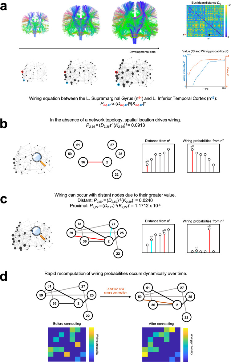
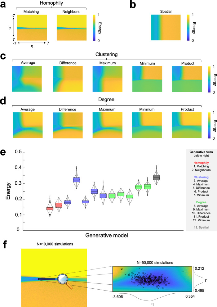
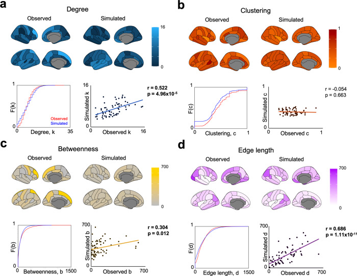
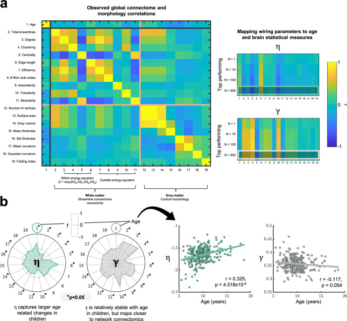
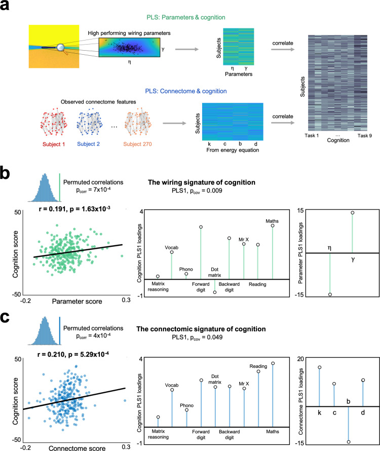
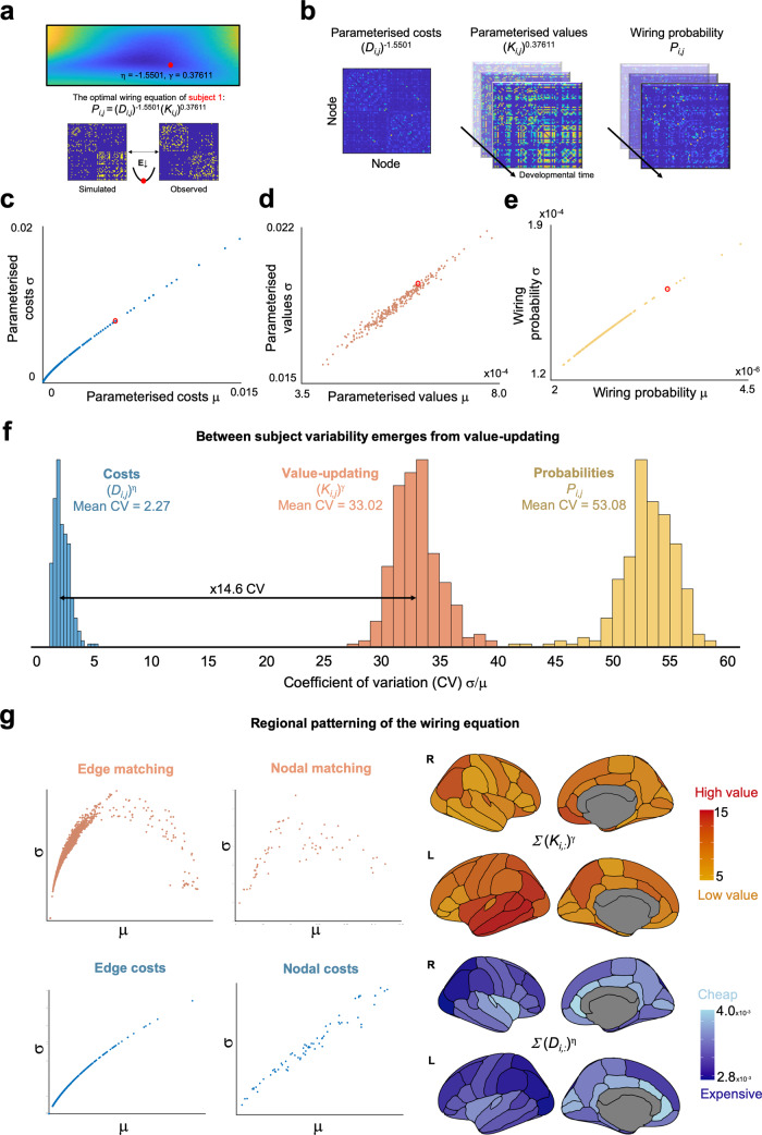
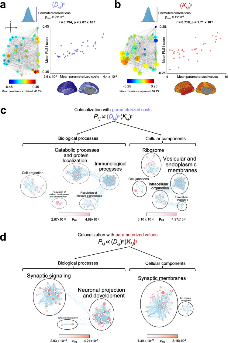
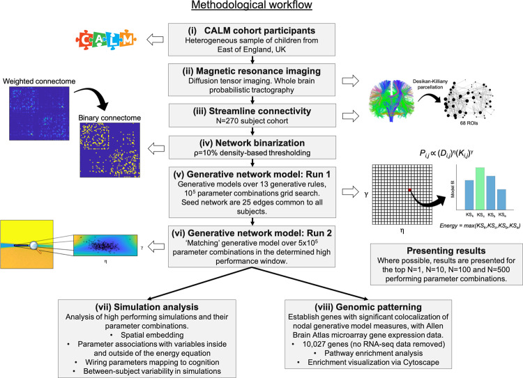
The formation of large-scale brain networks, and their continual refinement, represent crucial developmental processes that can drive individual differences in cognition and which are associated with multiple neurodevelopmental conditions. But how does this organization arise, and what mechanisms drive diversity in organization? We use generative network modeling to provide a computational framework for understanding neurodevelopmental diversity. Within this framework macroscopic brain organization, complete with spatial embedding of its organization, is an emergent property of a generative wiring equation that optimizes its connectivity by renegotiating its biological costs and topological values continuously over time. The rules that govern these iterative wiring properties are controlled by a set of tightly framed parameters, with subtle differences in these parameters steering network growth towards different neurodiverse outcomes. Regional expression of genes associated with the simulations converge on biological processes and cellular components predominantly involved in synaptic signaling, neuronal projection, catabolic intracellular processes and protein transport. Together, this provides a unifying computational framework for conceptualizing the mechanisms and diversity in neurodevelopment, capable of integrating different levels of analysis-from genes to cognition.

Fig. 1. Updating wiring probabilities within the generative network model iteratively, based on dynamically changing graphical structures.

a The brain’s structural connectivity is modeled as a generative network which grows over time according to parametrized connection costs, (D_i,j)^η and values, (K_i,j)^γ. In this illustration, we use subject one’s optimal model. b Early in network development, the absence of a topology leads to proximal nodes being much more likely to form connections. The displayed distances and probabilities are from the right caudal anterior cingulate (n²), which corresponds to row (D₂,:)^η and (P₂,:). We display it’s six nearest cortical regions. c Later, the relative values (K_i,j) between nodes influence connection probabilities, such that nodes which are more distant (e.g., left rostral anterior cingulate, n in red) may be preferred to nodes which are closer (e.g., right superior frontal cortex, n in cyan). d As costs and values are decoupled, the wiring probability can be rapidly recomputed when dynamic changes in graphical structure occur over developmental time.

Fig. 2. Sample-averaged energy landscape visualization and generative rule comparisons.

a Homophily-based methods. Matching and neighbors algorithms calculate a measure of shared neighborhood between nodes. b The spatial method. This ignores γ entirely, judging networks only on the basis of their spatial relationship. c Clustering-based methods. These calculate a summary measure between two nodes in terms of their clustering coefficients. d Degree-based methods. These calculate a summary measure between two nodes in terms of their degree. e Energy statistics from the best performing simulation across 13 generative rules, showing that matching can achieve the lowest energy networks given the appropriate parameter combination. In total, there are N = 270 data points for each of the 13 boxplots. A tabulated form of this figure is provided in Supplementary Table 1. The boxplot presents the median and IQR. Outliers are demarcated as small black crosses, and are those which exceed 1.5 times the interquartile range away from the top or bottom of the box. f A further 50,000 simulations were undertaken in the refined matching window, as these defined boundary conditions for which low-energetic networks were consistently achieved. Each cross represents a subject’s individually specific wiring parameters that achieved their lowest energy simulated network.

Fig. 3. Spatial embedding of simulated networks grown via optimized homophily generative mechanisms.

For each network measure, we present the cumulative density functions across all observed versus simulated nodes within each network. Each point in the scatter plot shows one of the 68 across-subject average nodal measures from the observed and optimally simulated networks. We also show a visualization of these measures. All statistics were computed via two-tailed linear correlations, quoting the Pearson’s correlation coefficient. a Degree between observed and simulations are significantly positively correlated (r = 0.522, p = 4.96 × 10⁻⁵). b Clustering between observed and simulations at not correlated (r = −0.054, p = 0.663). c Betweenness centrality between observed and simulations are significantly positively correlated (r = 0.304, p = 0.012). d Edge length (as a summation of all edges from each node) between observed and simulations are significantly positively correlated (r = 0.686, p = 1.11 × 10⁻¹¹). Boldened values are significant correlations at p < 0.05. In Supplementary Fig. 4, we present a parallel analysis including local and global measures not included in the energy equation. In Supplementary Fig. 5, we demarcate for each measure the generative error in spatial embedding, and show the ranked performance for each region.

Fig. 4. Statistical properties of the connectome and cortical morphology, and their relationships with wiring parameters and age.

a The correlation matrix of connectome and morphological findings show how each measure correlates with every other measure. Measures 3–6 were included in the energy equation. Measures 7–11 are connectome measures not included in the energy equation. Measures 12–19 are cortical morphological measures. η and γ are each significantly correlated with a range of measures, both inside and outside of the energy equation. Correlation coefficient matrices are shown, the bottom row of which is highlighted and is reflected in the above radar plots (middle), in addition to the significance matrix (bottom), across varying numbers of top performing parameters, for each of the 19 measures investigated. b Radar plots depict the correlations between all measures and η (left) and γ (right) averaged across the top N = 500 parameters in the parameter space. All statistics were computed via two-tailed linear correlations, quoting the Pearson’s correlation coefficient. The asterisk, *, reflects significant correlations at p < 0.05. Note, the inner edge of the radar plot reflects negative correlations and the outer edge reflects positive correlations. Specific results for variable top performing parameters are provided in Supplementary Table 3. Further scatter plots are provided highlighting the relationship of wiring parameters with age. η has a significantly positive relationship with age (r = 0.325, p = 4.518 × 10⁻⁸) while γ has a weak non-significant negative relationship with age (r = −0.117, p = 0.054).

Fig. 5. Covarying patterns of wiring parameters and connectome features with cognitive performance across nine cognitive tasks.

a A visual representation of the two PLS analyses undertaken. b There is a significant positive correlation (two-tailed linear correlation, quoting the Pearson’s correlation coefficient) between parameter scores and PLS-derived cognitive scores. PLS1 was statistically significant (p_corr = 7 × 10⁻⁴ and p_corr = 4 × 10⁻⁴, respectively) for both analyses using n = 10,000 permutations. Each parameter loads with similar magnitude onto PLS1. c There is an analogous significant positive correlation between connectome scores and PLS-derived cognition scores, using the same statistical procedure.

Fig. 6. Wiring Eq. (1) decomposition and the subsequent variability across subjects in our heterogeneous sample.

a For each subject, a simulated network is produced by minimizing the energy between the observed and simulated network. Here, we present visualizations for subject one (red). b Costs (D_i,j) are static, while values (K_i,j) dynamically update according to the matching rule, which enables the computation of wiring probability (P_i,j). c The mean and standard deviation for each subject of their edge-wise parameterized costs, d parameterized values and e wiring probabilities. f Histograms of each subject’s coefficient of variation (CV) showing that subjects are more variable in their value-updating compared to costs, leading to large wiring probability variability. g Regional patterning of sample-averaged nodal parameterized costs and values, showing highly “valuable” patterning in the left temporal lobe and “cheap” regions generally occupying medial aspects of the cortex. Variability declines as value increases, but increases for costs.

Fig. 7. Over expressed genes which explain variance in brain wiring across subjects.

Both PLS1 components across subjects are enriched for functionally specific biological processes and cellular components. Node size represents the number of genes in the set. The edges relate to gene overlap. a Sample-averaged parameterized costs significantly correlates with sample-averaged PLS1 nodal gene scores, explaining on average 65.0% covariance. Statistics were computed via two-tailed linear correlations, quoting the Pearson’s correlation coefficient, followed by n = 10,000 permutations. b Sample-averaged parameterized values significantly correlates with sample-averaged PLS1 nodal gene scores explaining on average 56.9% covariance. Statistics were computed via two-tailed linear correlations, quoting the Pearson’s correlation coefficient, followed by n = 10,000 permutations. c Nodal costs PLS1 is enriched for genes predominantly associated with protein localization, catabolic processes, and ribosomal/membrane cellular components. d Nodal values PLS1 is enriched for genes predominantly associated with synaptic signaling, neuronal projection and synaptic membranes.

Fig. 8. Schematic of the methodological workflow.

The basic workflow involved (i) Recruitment of the CALM cohort, a heterogeneous referred sample from the East of England (UK) with wide inclusion criteria; (ii) MRI diffusion tensor imaging; (iii) Estimation of structural connectivity within the Desikan–Killiany parcellation; (iv) Binarization of the connectome; (v) Initial run of the GNM for all 13 generative rules as outlined in Supplementary Table 1; (vi) More specific run of the homophily “matching” GNM in the narrow parameter window; (vii) Further analysis of simulations in terms of spatial embedding, parameter associations and variability; (viii) Combination of Allen Human Brain Atlas data and the generative model findings.

References

1. Basser PJ, Pajevic S, Pierpaoli C, Duda J, Aldroubi A. In vivo fiber tractography using DT-MRI data. Magn. Reson. Med. 2000;44:625–632. doi: 10.1002/1522-2594(200010)44:4<625::AID-MRM17>3.0.CO;2-O. - DOI - PubMed
1. Conturom TE, et al. Tracking neuronal fiber pathways in the living human brain. Proc. Natl Acad. Sci. USA. 1999;96:10422–10427. doi: 10.1073/pnas.96.18.10422. - DOI - PMC - PubMed
1. Mori S, Crain BJ, Chacko VP, van Zijl PC. Three-dimensional tracking of axonal projections in the brain by magnetic resonance imaging. Ann. Neurol. 1999;45:265–269. doi: 10.1002/1531-8249(199902)45:2<265::AID-ANA21>3.0.CO;2-3. - DOI - PubMed
1. Friston K. Functional integration and inference in the brain. Prog. Neurobiol. 2002;68:113–143. doi: 10.1016/S0301-0082(02)00076-X. - DOI - PubMed
1. Mahon BZ, Cantlon JF. The specialization of function: cognitive and neural perspectives. Cogn. Neuropsychol. 2011;28:147–155. doi: 10.1080/02643294.2011.633504. - DOI - PMC - PubMed
Publication types