Tree-aggregated predictive modeling of microbiome data

Abstract

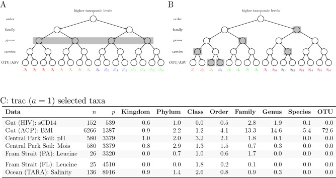
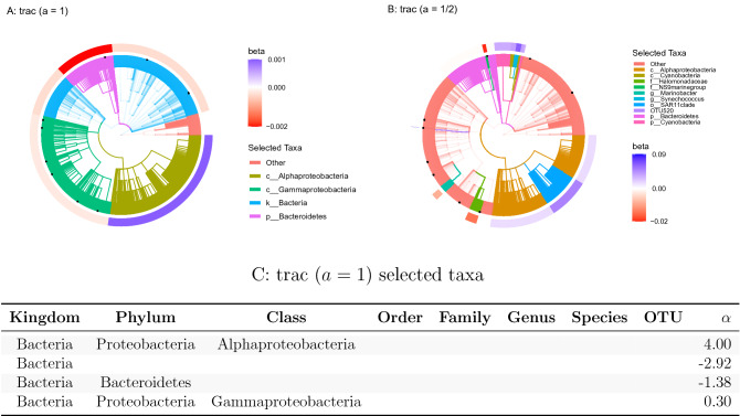
Modern high-throughput sequencing technologies provide low-cost microbiome survey data across all habitats of life at unprecedented scale. At the most granular level, the primary data consist of sparse counts of amplicon sequence variants or operational taxonomic units that are associated with taxonomic and phylogenetic group information. In this contribution, we leverage the hierarchical structure of amplicon data and propose a data-driven and scalable tree-guided aggregation framework to associate microbial subcompositions with response variables of interest. The excess number of zero or low count measurements at the read level forces traditional microbiome data analysis workflows to remove rare sequencing variants or group them by a fixed taxonomic rank, such as genus or phylum, or by phylogenetic similarity. By contrast, our framework, which we call trac (tree-aggregation of compositional data), learns data-adaptive taxon aggregation levels for predictive modeling, greatly reducing the need for user-defined aggregation in preprocessing while simultaneously integrating seamlessly into the compositional data analysis framework. We illustrate the versatility of our framework in the context of large-scale regression problems in human gut, soil, and marine microbial ecosystems. We posit that the inferred aggregation levels provide highly interpretable taxon groupings that can help microbiome researchers gain insights into the structure and functioning of the underlying ecosystem of interest.

Figure 1

Illustration of fixed level and trac-based taxon aggregation. The trees represent the available taxonomic grouping of 16 base level taxa at the leaves (here OTU or ASV). (A) Arithmetic aggregation of OTUs/ASVs to a fixed level (genus rank). All taxon base level counts are summed up to the respective parent genus. (B) trac’s flexible tree-based aggregation in which the choice of what level to aggregate to can vary across the tree (e.g., two OTUs/ASVs, two species, one genus, and one family). The aggregation is based on the geometric mean of OTU/ASV counts and determined in a data-adaptive fashion with the goal of optimizing to the particular prediction task. (C) Summary statistics of standard trac-inferred aggregation levels on all seven regression tasks. The Data column denotes the respective regression scenario (study name and outcome of interest), n the number of samples, and p the number of base level taxa (OTUs) in the data. The values in the taxonomic rank columns (Kingdom, Phylum, etc.) indicate the average number of taxa selected on that level by trac  in the respective regression task. Averages are taken over ten random training/out-of-sample test data splits.

Figure 2

Overview of trac aggregation and model selection with standard weighting $a=1$ on the sCD14 data. (A) Varying the trac regularization parameter $\lambda$ produces a solution (aggregation) path. Each colored line corresponds to a distinct taxon, showing its $\alpha$ coefficient value as the tuning parameter $\lambda$ increases. The larger $\lambda$ is, the more coefficients are set to 0, leading to a more parsimonious model. The dotted and dashed vertical lines mark the $\lambda$-values selected by the CV best and 1SE rule, respectively. (B) Illustration of the cross-validation (CV) procedure. Mean (and standard error) CV error vs. $\lambda$ path with selected $\lambda$ values at best CV error (dotted vertical line) or with the 1SE rule (dashed vertical line). (C) The actual vs. predicted values of sCD14 on the test set (1SE rule in red, CV best in blue). The Pearson correlation of trac predictions on the test set is 0.37 with the CV best solution and 0.23 with the CV 1SE rule, respectively. (D) Error on the test set vs. number of selected aggregations. (E) The trac model selected with the 1SE rule comprises five taxa across four levels, listed in the bottom table (see Fig. 3A for tree visualization of the aggregations). The column labeled $\alpha$ gives the nonzero coefficient values, which are in the same units as the sCD14 response variable.

Figure 3

Taxonomic tree visualization of trac aggregations in four selected scenarios using sCD14 data (training/test split 1). Each tree represents the taxonomy of the $p=539$ OTUs. Colored branches highlight the estimated trac taxon aggregations. The black dots mark the selected taxa of the respective sparse log-contrast model. The outer rim represents the value of $\beta$ coefficients in the trac  model from Eq. (1). (A) Standard trac ($a=1$) with OTUs as taxon base level selects five aggregations. (B) Weighted trac ($a=1/2$) with OTU base level selects eleven aggregations, including six on the OTU level. Four of these OTUs were also selected by the sparse log-contrast model which comprises nine OTUs in total (black dots) (see Suppl. Tables 6 and 7 for the selected coefficients). (C) Standard trac ($a=1$) with family base level selects three aggregations. (D) Weighted trac ($a=1/2$) with family as taxon base level selects five aggregations, including one family (Enterobacteriacaeae) shared with the sparse log-contrast model when also applied at the family base level (see Suppl. Tables 10 for the six selected families).

Figure 4

Taxonomic tree visualization of trac aggregations ($a\in \{1,1/2\}$ using the Central Park soil data (training/test split 1). Each tree represents the taxonomy of the $p=3379$ OTUs. Colored branches highlight the estimated trac taxon aggregations. The black dots mark the selected taxa of the sparse log-contrast model. The outer rim represents the value of $\beta$ coefficients in the trac model from Eq. (1). (A) Standard trac ($a=1$) with OTUs as taxon base level selects six aggregations. (B) Weighted trac ($a=1/2$) with OTU base level selects 28 aggregations, including 13 on the OTU level. Four of these OTUs are also selected by the sparse log-contrast model which comprises 21 OTUs in total (black dots) (see Suppl. Tables 15 and 16 for the selected coefficients). (C) The table lists the $\alpha$ coefficients associated with Eq. (2) for the trac ($a=1$) model corresponding to the tree shown in (A). These values are in the same units as the pH response variable.

Figure 5

Taxonomic tree visualization of trac aggregations (OTUs as taxon base level, $a\in \{1,1/2\}$ for salinity prediction using Tara data (training/test split 1). Each tree represents the taxonomy of the $p=8916$ miTAG OTUs. Colored branches highlight the estimated trac taxon aggregations. The black dots mark the selected taxa of the sparse log-contrast model. The outer rim represents the value of $\beta$ coefficients in the trac model from Eq. (1). (A) Standard trac ($a=1$) selects four aggregations on the kingdom, phylum, and class level. (B) Weighted trac ($a=1/2$) selects ten aggregations across all taxonomic ranks, including a single OTU (OTU520). This OTU is also selected by the sparse log-contrast model which comprises nine OTUs in total (black dots) (see Suppl. Table 18 for the selected coefficients). Both trac models select the phylum Bacteroidetes and the Alphaproteobacteria class. (C) The table lists the $\alpha$ coefficients associated with Eq. (2) for the trac ($a=1$) model corresponding to the tree shown in ( A). These values are in the same units as the salinity response variable.

References

1. Sender R, Fuchs S, Milo R. Revised estimates for the number of human and bacteria cells in the body. PLoS Biol. 2016;14(8):1–14. doi: 10.1371/journal.pbio.1002533. - DOI - PMC - PubMed
1. Bar-On YM, Phillips R, Milo R. The biomass distribution on Earth. Proc. Natl. Acad. Sci. USA. 2018;115(25):6506–6511. doi: 10.1073/pnas.1711842115. - DOI - PMC - PubMed
1. Sunagawa, S. et al. Structure and function of the global ocean microbiome. Science348(6237) (2015). - PubMed
1. Bahram, M. et al. Structure and function of the global topsoil microbiome. Nature560(7717), 233–237 (2018). - PubMed
1. McDonald, D. et al. American gut: An open platform for citizen science microbiome research. mSystems3(3) (2018). - PMC - PubMed
Publication types