. 2021 Jul 19;19(7):e3001347.
doi: 10.1371/journal.pbio.3001347. eCollection 2021 Jul.

Do psychiatric diseases follow annual cyclic seasonality?

Affiliations

Do psychiatric diseases follow annual cyclic seasonality?

Hanxin Zhang et al. PLoS Biol. .

Abstract

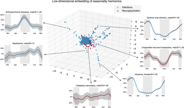
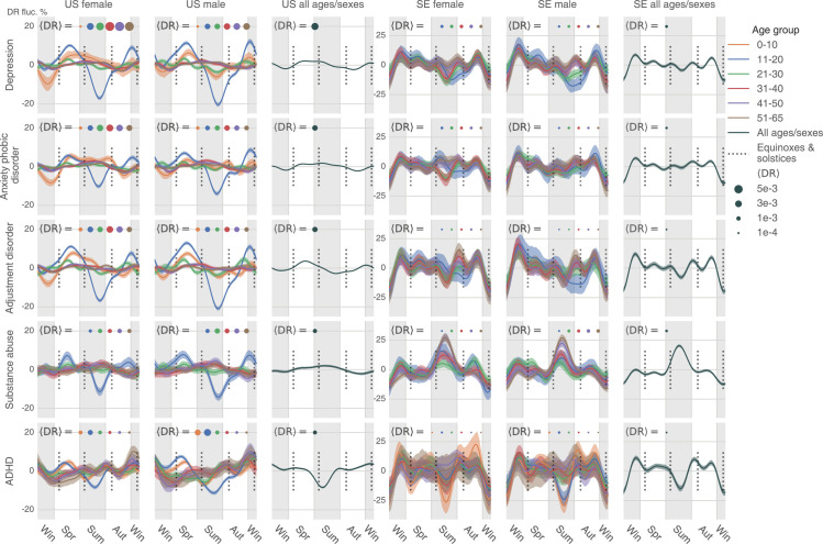
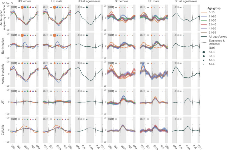
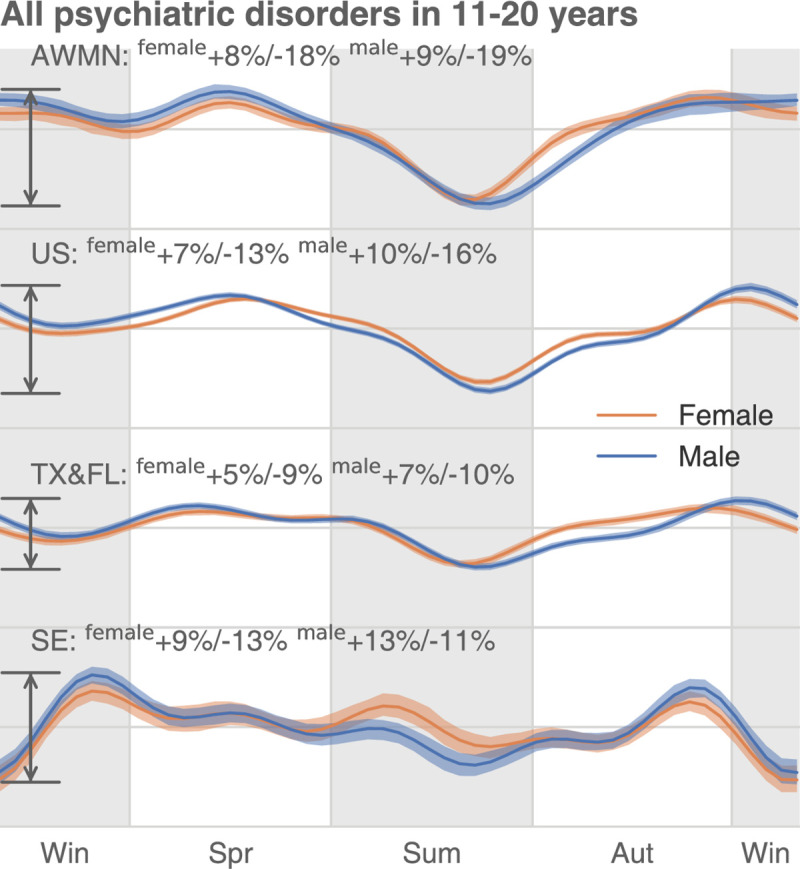
Seasonal affective disorder (SAD) famously follows annual cycles, with incidence elevation in the fall and spring. Should some version of cyclic annual pattern be expected from other psychiatric disorders? Would annual cycles be similar for distinct psychiatric conditions? This study probes these questions using 2 very large datasets describing the health histories of 150 million unique U.S. citizens and the entire Swedish population. We performed 2 types of analysis, using "uncorrected" and "corrected" observations. The former analysis focused on counts of daily patient visits associated with each disease. The latter analysis instead looked at the proportion of disease-specific visits within the total volume of visits for a time interval. In the uncorrected analysis, we found that psychiatric disorders' annual patterns were remarkably similar across the studied diseases in both countries, with the magnitude of annual variation significantly higher in Sweden than in the United States for psychiatric, but not infectious diseases. In the corrected analysis, only 1 group of patients-11 to 20 years old-reproduced all regularities we observed for psychiatric disorders in the uncorrected analysis; the annual healthcare-seeking visit patterns associated with other age-groups changed drastically. Analogous analyses over infectious diseases were less divergent over these 2 types of computation. Comparing these 2 sets of results in the context of published psychiatric disorder seasonality studies, we tend to believe that our uncorrected results are more likely to capture the real trends, while the corrected results perhaps reflect mostly artifacts determined by dominantly fluctuating, health-seeking visits across a given year. However, the divergent results are ultimately inconclusive; thus, we present both sets of results unredacted, and, in the spirit of full disclosure, leave the verdict to the reader.


Conflict of interest statement

The authors have declared that no competing interests exist.

Figures

Fig 1
Fig 1. The characteristics of the US data and how it influences our model design.
(A) Our modeling aimed to correct biases and noise in the MarketScan database and to infer a latent disease DR trend and seasonality for specific age–sex groups. The upper left panel describes the scenario in which 2 populations—a healthy one (the blue line) and an unhealthy one (the red line)—enrolled in the data at different times. The blue and red lines represent the trend of the DR for the 2 populations. We can see that the healthy population joined and left our data earlier than the unhealthy one. Thus, if we fit a simple linear regression model, the result may lead us to conclude that there is an upward trend of DR. Nonetheless, the real trend is actually constant if we had the ability to collect the data of all time (synchronous enrollment) for both populations. The trend of the linear fit (the orange line) comes from “asynchronous enrollments” of populations in various health statuses. The rest of the panels delineate other scenarios likewise. (B) This subplot shows the overall trend and seasonality for a sample disease. The holiday-smooth function offsets the effect of holidays and celebrations that decrease the DR sharply (the orange curve vs. the blue curve). Bear in mind that patients joined and left our US data asynchronously. The gray lines illustrate varying linear fit trends of population strata, defined according to their enrollment dates (see the Methods and techniques part of the Materials and methods section). Some population strata include more people, while others are smaller in size, as marked by the gray lines’ different widths. A sample population stratum enrolled from week 1 to 195 is highlighted in the right panel. Notice that the sudden shift still exists—even for a population with a consistent composition, meaning that the shifts do not result from enrollment changes. The data underlying this figure can be found in https://doi.org/10.5061/dryad.vdncjsxv6. DR, diagnosis rate.
Fig 2
Fig 2. The method and procedure to infer seasonality.
Upper frame (Step 1): We modeled the DR by decomposing it into several parts: the linear trend, yearly shifts, seasonality, and an error term. We assigned people into hundreds of population strata according to their enrollment dates. A total of 6 populations of specific age and enrollment dates are shown here. The model fits each population strata separately (but not independently), with shared priors and hyperpriors so that information can be shared across populations. “In” means the time the stratum joined our data (enrollment beginning), and “Out” indicates the time they left (enrollment end). Lower frame (Step 2): After obtaining the estimates of all model parameters, we were able to extract the seasonality and make inferences. The upper plot shows that the posterior expectation (mean) reproduces our raw observation very well, which partly validates that our model is mixing well. Note that, for this particular condition, the 95% highest posterior density interval is very small, so it may be difficult to tell it in the plot (light green shade). The left subplot at the bottom exemplifies how we can find the relative seasonal fluctuation (uncorrected) s(t) by dividing the seasonality estimates by the time-average DR (〈DR〉, Expression (17)). We can possibly correct for the baseline fluctuation of all medical visits by deducting the sall(t) (representing the uncorrected seasonality of all medical visits) from s(t) and obtain the corrected seasonality s′(t) (right subplot at the bottom). The data underlying this figure can be found in https://doi.org/10.5061/dryad.vdncjsxv6. DR, diagnosis rate.
Fig 3
Fig 3. The uncorrected seasonality plots of the 5 most diagnosed psychiatric diseases in the US: Depression, anxiety/phobic disorder, adjustment disorder, substance abuse, and ADHD.
The results in SE are juxtaposed, but scaled by 0.3 in magnitude for clearer comparison. We plotted all lines based on a weekly DR estimated as the total number of diagnoses in a week, divided by the total number of enrollees in our database in the week. Positive and negative maximum fluctuations compared to the mean DR are text-labeled following a format: Country female maximum fluctuation in percentage / Male max fluctuation in percentage. We use the meteorological seasons defined as follows: Winter starts from December 1 and ends on February 28, spring starts from March 1 and ends on May 31, summer starts from June 1 and ends on August 31, and autumn is the rest of the year. We discarded the health records of people over 65 because the majority of that population in the US data switched to Medicare, and remaining records were not representative. A disease could be extremely rare in some age–sex brackets. The plot only shows those age–sex–specific seasonalities with a time-average DR (Expression (17)) larger than 1×10⁻⁵. The data underlying this figure can be found in https://doi.org/10.5061/dryad.vdncjsxv6. ADHD, attention-deficit/hyperactivity disorder; DR, diagnosis rate; SE, Sweden.
Fig 4
Fig 4. The uncorrected seasonality plots of the 5 most diagnosed infectious diseases in the US: Acute upper respiratory infection, ear infection, acute bronchitis, UTI, and cellulitis.
The results in SE are juxtaposed without scaling. A disease could be extremely rare in some age–sex brackets. The plot only shows those age–sex–specific seasonalities with a time-average DR larger than 1×10⁻⁵. The data underlying this figure can be found in https://doi.org/10.5061/dryad.vdncjsxv6. DR, diagnosis rate; SE, Sweden; UTI, urinary tract infection.
Fig 5
Fig 5. The embedding of uncorrected seasonality curves in a low-dimensional space suggests the homogeneity of the psychiatric diseases’ seasonal variation.
We used the Isomap method to obtain a low-dimensional seasonality embedding of the first 10 Fourier harmonic base estimates p¯j,1,p¯j,2, …, p¯j,5,q¯j,1,q¯j,2, …, q¯j,5 (see Expressions (15) and (16)). Compared to the infectious diseases, we can see that the embeddings of psychiatric disease harmonics concentrate in a smaller space, implying the relative homogeneity of their seasonality. The data underlying this figure can be found in https://doi.org/10.5061/dryad.vdncjsxv6.
Fig 6
Fig 6. The corrected seasonality plots of the 5 most diagnosed psychiatric diseases in the US and SE: Depression, anxiety and phobic disorder, adjustment disorder, substance abuse, and ADHD. ADHD, attention-deficit/hyperactivity disorder; DR, diagnosis rate; SE, Sweden.
Fig 7
Fig 7. The corrected seasonality plots of the 5 most diagnosed infectious diseases in the US and SE: acute upper respiratory infection, ear infection, acute bronchitis, UTI, and cellulitis.
The data underlying this figure can be found in https://doi.org/10.5061/dryad.vdncjsxv6. DR, diagnosis rate; SE, Sweden; UTI, urinary tract infection.
Fig 8
Fig 8. The corrected seasonality of all psychiatric disorders in 11 to 20 year olds across 4 regions.
In the US, the annual oscillation of psychiatric disease DR is larger in the high-latitude areas (AK, WA, MT, ND, or AWMN) than in the low-latitude areas (TX and FL). The data underlying this figure can be found in https://doi.org/10.5061/dryad.vdncjsxv6. AK, Alaska; AWMN, Alaska, Washington, Montana, North Dakota; DR, diagnosis rate; MT, Montana; ND, North Dakota; WA, Washington.

Similar articles

Cited by

References

    1. Brainstorm Consortium, Anttila V, Bulik-Sullivan B, Finucane HK, Walters RK, Bras J, et al.. Analysis of shared heritability in common disorders of the brain. Science. 2018;360(6395). Epub 2018/06/23. doi: 10.1126/science.aap8757 . - DOI - PMC - PubMed
    1. Solberg BS, Zayats T, Posserud MB, Halmoy A, Engeland A, Haavik J, et al.. Patterns of Psychiatric Comorbidity and Genetic Correlations Provide New Insights Into Differences Between Attention-Deficit/Hyperactivity Disorder and Autism Spectrum Disorder. Biol Psychiatry. 2019;86(8):587–98. Epub 2019/06/12. doi: 10.1016/j.biopsych.2019.04.021 ; PubMed Central PMCID: PMC6764861. - DOI - PMC - PubMed
    1. Tylee DS, Sun J, Hess JL, Tahir MA, Sharma E, Malik R, et al.. Genetic correlations among psychiatric and immune-related phenotypes based on genome-wide association data. Am J Med Genet B Neuropsychiatr Genet. 2018;177(7):641–57. Epub 2018/10/17. doi: 10.1002/ajmg.b.32652 ; PubMed Central PMCID: PMC6230304. - DOI - PMC - PubMed
    1. Wen Y, Zhang F, Ma X, Fan Q, Wang W, Xu J, et al.. eQTLs Weighted Genetic Correlation Analysis Detected Brain Region Differences in Genetic Correlations for Complex Psychiatric Disorders. Schizophr Bull. 2019;45(3):709–15. Epub 2018/06/19. doi: 10.1093/schbul/sby080 ; PubMed Central PMCID: PMC6483588. - DOI - PMC - PubMed
    1. Jia G, Li Y, Zhang H, Chattopadhyay I, Boeck Jensen A, Blair DR, et al.. Estimating heritability and genetic correlations from large health datasets in the absence of genetic data. Nat Commun. 2019;10(1):5508. Epub 2019/12/05. doi: 10.1038/s41467-019-13455-0 ; PubMed Central PMCID: PMC6890770. - DOI - PMC - PubMed

Publication types