

Understanding the thermodynamic properties of insect swarms
- PMID: 34294865
- PMCID: PMC8298516
- DOI: 10.1038/s41598-021-94582-x
Understanding the thermodynamic properties of insect swarms
Abstract
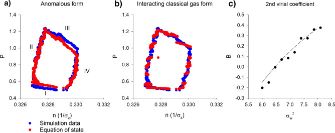
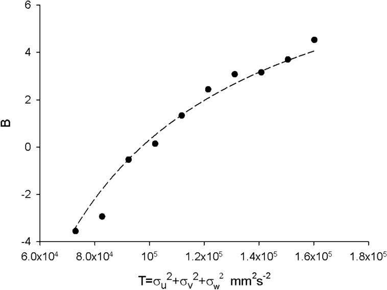
Sinhuber et al. (Sci Rep 11:3773, 2021) formulated an equation of state for laboratory swarms of the non-biting midge Chironomus riparius that holds true when the swarms are driven through thermodynamic cycles by the application external perturbations. The findings are significant because they demonstrate the surprising efficacy of classical equilibrium thermodynamics for quantitatively characterizing and predicting collective behaviour in biology. Nonetheless, the equation of state obtained by Sinhuber et al. (2021) is anomalous, lacking a physical analogue, making its' interpretation problematic. Moreover, the dynamical processes underlying the thermodynamic cycling were not identified. Here I show that insect swarms are equally well represented as van der Waals gases and I attribute the possibility of thermodynamic cycling to insect swarms consisting of several overlapping sublayers. This brings about a profound change in the understanding of laboratory swarms which until now have been regarded as consisting of non-interacting individuals and lacking any internal structure. I show how the effective interactions can be attributed to the swarms' internal structure, the external perturbations and to the presence of intrinsic noise. I thereby show that intrinsic noise which is known to be crucial for the emergence of the macroscopic mechanical properties of insect swarms is also crucial for the emergence of their thermodynamic properties as encapsulated by their equation of state.
© 2021. The Author(s).
Conflict of interest statement
The authors declare no competing interests.
Figures
Similar articles
-
An equation of state for insect swarms.Sci Rep. 2021 Feb 12;11(1):3773. doi: 10.1038/s41598-021-83303-z. Sci Rep. 2021. PMID: 33580191 Free PMC article.
-
Environmental perturbations induce correlations in midge swarms.J R Soc Interface. 2020 Mar;17(164):20200018. doi: 10.1098/rsif.2020.0018. Epub 2020 Mar 25. J R Soc Interface. 2020. PMID: 32208820 Free PMC article.
-
On the tensile strength of insect swarms.Phys Biol. 2016 Aug 25;13(4):045002. doi: 10.1088/1478-3975/13/4/045002. Phys Biol. 2016. PMID: 27559838
-
Dynamical aspects of animal grouping: swarms, schools, flocks, and herds.Adv Biophys. 1986;22:1-94. doi: 10.1016/0065-227x(86)90003-1. Adv Biophys. 1986. PMID: 3551519 Review.
-
Microscopic Swarms: From Active Matter Physics to Biomedical and Environmental Applications.Micromachines (Basel). 2022 Feb 13;13(2):295. doi: 10.3390/mi13020295. Micromachines (Basel). 2022. PMID: 35208419 Free PMC article. Review.
Cited by
-
Ontogeny of collective behaviour.Philos Trans R Soc Lond B Biol Sci. 2023 Apr 10;378(1874):20220065. doi: 10.1098/rstb.2022.0065. Epub 2023 Feb 20. Philos Trans R Soc Lond B Biol Sci. 2023. PMID: 36802780 Free PMC article. Review.
-
Insights and challenges of insecticide resistance modelling in malaria vectors: a review.Parasit Vectors. 2024 Apr 3;17(1):174. doi: 10.1186/s13071-024-06237-1. Parasit Vectors. 2024. PMID: 38570854 Free PMC article. Review.
-
Mosquito swarms shear harden.Eur Phys J E Soft Matter. 2023 Dec 8;46(12):126. doi: 10.1140/epje/s10189-023-00379-3. Eur Phys J E Soft Matter. 2023. PMID: 38063901 Free PMC article.
References
-
- Ouellette NT. Toward a ‘thermodynamics’ of collective behavior. SIAM News. 2017;40:1–4.
-
- Ouellette NT. The most active matter of all. Matter. 2019;1:297–299. doi: 10.1016/j.matt.2019.07.012. - DOI
-
- Peleg O, Peters JM, Salcedo MK, Mahadevan L. Collective mechanical adaptation of honeybee swarms. Nat. Phys. 2018;14:1193–1198. doi: 10.1038/s41567-018-0262-1. - DOI
Publication types
MeSH terms
Grants and funding
LinkOut - more resources
Full Text Sources
