. 2019:7:372.
doi: 10.3389/fevo.2019.00372. Epub 2019 Oct 21.

Errors in Statistical Inference Under Model Misspecification: Evidence, Hypothesis Testing, and AIC

Affiliations

Errors in Statistical Inference Under Model Misspecification: Evidence, Hypothesis Testing, and AIC

Brian Dennis et al. Front Ecol Evol. 2019.

Abstract

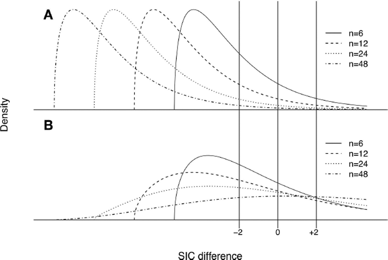
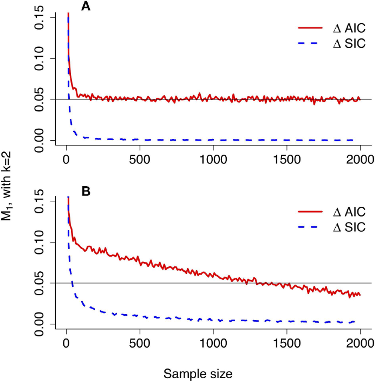
The methods for making statistical inferences in scientific analysis have diversified even within the frequentist branch of statistics, but comparison has been elusive. We approximate analytically and numerically the performance of Neyman-Pearson hypothesis testing, Fisher significance testing, information criteria, and evidential statistics (Royall, 1997). This last approach is implemented in the form of evidence functions: statistics for comparing two models by estimating, based on data, their relative distance to the generating process (i.e., truth) (Lele, 2004). A consequence of this definition is the salient property that the probabilities of misleading or weak evidence, error probabilities analogous to Type 1 and Type 2 errors in hypothesis testing, all approach 0 as sample size increases. Our comparison of these approaches focuses primarily on the frequency with which errors are made, both when models are correctly specified, and when they are misspecified, but also considers ease of interpretation. The error rates in evidential analysis all decrease to 0 as sample size increases even under model misspecification. Neyman-Pearson testing on the other hand, exhibits great difficulties under misspecification. The real Type 1 and Type 2 error rates can be less, equal to, or greater than the nominal rates depending on the nature of model misspecification. Under some reasonable circumstances, the probability of Type 1 error is an increasing function of sample size that can even approach 1! In contrast, under model misspecification an evidential analysis retains the desirable properties of always having a greater probability of selecting the best model over an inferior one and of having the probability of selecting the best model increase monotonically with sample size. We show that the evidence function concept fulfills the seeming objectives of model selection in ecology, both in a statistical as well as scientific sense, and that evidence functions are intuitive and easily grasped. We find that consistent information criteria are evidence functions but the MSE minimizing (or efficient) information criteria (e.g., AIC, AICc, TIC) are not. The error properties of the MSE minimizing criteria switch between those of evidence functions and those of Neyman-Pearson tests depending on models being compared.

Keywords: Akaike’s information criterion; Kullback-Leibler divergence; error rates in model selection; evidence; evidential statistics; hypothesis testing; model misspecification; model selection.


Conflict of interest statement

Conflict of Interest: The authors declare that the research was conducted in the absence of any commercial or financial relationships that could be construed as a potential conflict of interest.

Figures

FIGURE 1 |
FIGURE 1 |
Model topologies when models are correctly specified. Regions represent parameter spaces. Star represents the true parameter value corresponding to the model that generated the data. Top: a nested configuration would occur, for example, in the case of two regression models if the first model had predictor variables R1 and R2 while the second had predictor variables R1, R2, and R3. Middle: an overlapping configuration would occur if the first model had predictor variables R1 and R2 while the second had predictor variables R2 and R3. Three locations of truth are possible: truth in model 1, truth in model 2, and truth in both models 1 and 2. Bottom: an example of a non-overlapping configuration is when the first model has predictor variables R1 and R2 while the second model has predictor variables R3 and R4.
FIGURE 2 |
FIGURE 2 |
Model topologies when models are misspecified. Regions represent parameter spaces. Star represents the true model that generated the data. Exes represent the point in the parameter space covered by the model set closest to the true generating process.
FIGURE 3 |
FIGURE 3 |
Evidence error probabilities for comparing two Bernoulli(p) distributions, with p1 = 0.75 and p2 = 0.50. (A) Simulated values (jagged curve) and values approximated under the Central Limit Theorem of the probability of strong evidence for model H1, V1 = 1 − M1W1. (B) Simulated values (jagged curve) and approximated values for the probability of misleading evidence M1. Note that the scale of the bottom graph is one fifth of that of the top graph.
FIGURE 4 |
FIGURE 4 |
Four model configurations involving a bivariate generating process g(x1, x2) (in black), and two approximating models f1(x1, x2) (in blue) and f2(x1, x2) (in red). In all cases the approximating models are bivariate normal distributions whereas the generating process is a bivariate Laplace distribution. These model configurations are useful to explore changes in α′ (Equation 53), β′ (Equation 59) and Mi,Wi,i=1,2 (Equations 71, 72) as a function of sample size, as plotted in Figure 6. (A) g(x1, x2) is a bivariate Laplace distribution centered at 0 with high variance. All three models have means aligned along the 1: 1 line and marked with a black, blue, and red filled circle, respectively. Model f1(x1, x2) is closest to the generating process. (B) Model f1(x1, x2) is still the model closest to the generating process, at exactly the same distance as in (A) but misaligned from the 1: 1 line. (C) Here all three models are again aligned, but the generating process g(x1, x2) is an asymmetric bivariate Laplace that has a large mode at 0, 0 and smaller mode around the mean, marked with a black dot. In this case, the generating model is closer to model f2(x1, x2) (in red). (D) Same as in (C), except model f2(x1, x2) (in blue) is now misaligned, but still the closest model to the generating process.
FIGURE 5 |
FIGURE 5 |
Changes in α′ (Equation 53), β′ (Equation 59) and Mi,Wi,i=1,2 (Equations 71, 72) as a function of sample size. The plot in (A–D) were computed under each of the geometries plotted in Figures 4A–D. (A) α′, M1, and W1 for the models geometry in Figure 4A, where all models are aligned and model f1 is closest to the generating process. (B) Same as in (A) but model f1 is misaligned. C β′, M2, and W2 for model geometry in Figure 4C, where model f2 is closer to the generating process and all models are aligned. D: β′, M2, and W2 for model geometry in Figure 4D, where model f2 is closer to the generating process but model f2 is misaligned.
FIGURE 6 |
FIGURE 6 |
Evidence error probabilities for comparing two Bernoulli(p) distributions, with p1 = 0.75 and p2 = 0.50, when the true data-generating model is Bernoulli with p = 0.65. (A) Simulated values (jagged curve) and values approximated under the Central Limit Theorem of the probability (α′) of rejecting model H1 when it is closer than H2 to the true model. (B) Simulated values (jagged curve) and approximated values for the probability (M1) of misleading evidence for model H2 when model H1 is closer to the true data-generating process.
FIGURE 7 |
FIGURE 7 |
Moment of discovery: page from Professor H. Akaike’s research notebook, written while he was commuting on the train in March 1971. Photocopy kindly provided by the Institute for Statistical Mathematics, Tachikawa, Japan.
FIGURE 8 |
FIGURE 8 |
(A) Location-shifted chisquare distribution of the difference of AIC values, when data arise from model 1 nested within model 2. In this plot, the degrees of freedom for this distribution are equal to ν = 3, and the shift to the left of 0 is equal 2ν = 6 (see Equation 77 and text below it). This chisquare distribution is invariant to sample size. As a result, the areas under this distribution in the intervals (−2, +2) and (+2, ∞) corresponding to W1 and M1, respectively, are invariant to sample size. (B) Non-central chisquare distribution of the difference of AIC values, when data arise from model 2 (but not model 1), plotted for different sample sizes. This distribution is also location-shifted but its non-centrality parameter λ, which determines both its mean and variance, is proportional to sample size. In this illustration, λ = n(1/4). As a result, the areas under the intervals (−2ν, −2) and (−2, +2) corresponding to the error probabilities M2 and W2 decrease as the sample size increases.
FIGURE 9 |
FIGURE 9 |
(A) Chisquare distribution of the difference of SIC values, when data arise from model 1 nested within model 2. The chisquare distribution is shifted left as sample size increases. (B) Non-central chisquare distribution of the difference of SIC values, when data arise from model 2 (but not model 1), plotted for increasing sample sizes.
FIGURE 10 |
FIGURE 10 |
Simulation of Vuong (1989) results for misspecified models. (A) When f1 (x, θ1*) and f2 (x, θ2*) are the same model (either f1 is nested within f2, or f1 overlaps f2, and the best model is in the nested or overlapping region), then the asymptotic distribution of G2 is a “weighted sum of chisquares” that does not depend on n. The error probabilities M1 and W1 do not decrease to 0 for ΔAIC12 but do decrease for ΔSIC12. (B) When the models are nested, overlapping, or non-overlapping, but a non-overlapping part of f1 or f2 is closer to truth, then G2 has an asymptotic normal distribution with mean and variance that depend on the sample size, and the error probabilities M1 and W1 decrease to 0 for both ΔAIC12 and ΔSIC12. Details of these two settings in (A,B) are found in a fully commented R code.

References

    1. Aho K, Derryberry D, and Peterson T (2014). Model selection for ecologists: the worldviews of AIC and BIC. Ecology 95, 631–636. doi: 10.1890/13-1452.1 - DOI - PubMed
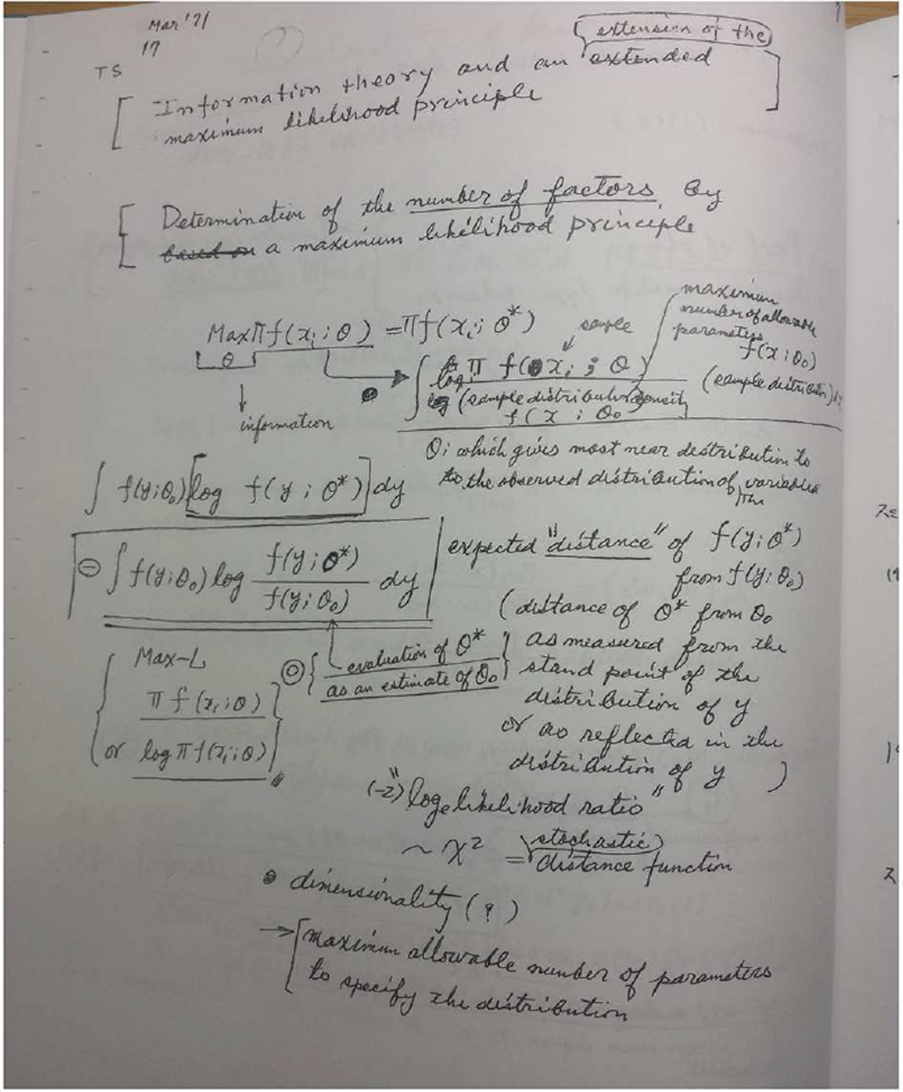
    1. Akaike H (1973). “Information theory as an extension of the maximum likelihood principle,” in Second International Symposium on Information Theory, eds Petrov B, and Csaki F (Budapest: Akademiai Kiado; ), 267–281.
    1. Akaike H (1974). A new look at statistical-model identification. IEEE Trans. Autom. Control 19, 716–723. doi: 10.1109/TAC.1974.1100705 - DOI
    1. Akaike H (1981). Likelihood of a model and information criteria. J. Econ 16, 3–14. doi: 10.1016/0304-4076(81)90071-3 - DOI
    1. Anderson D, Burnham K, and Thompson W (2000). Null hypothesis testing: problems, prevalence, and an alternative. J. Wildl. Manag 64, 912–923. doi: 10.2307/3803199 - DOI

LinkOut - more resources