. 2021 Jul 8:12:645640.
doi: 10.3389/fgene.2021.645640. eCollection 2021.

Exact Probability Landscapes of Stochastic Phenotype Switching in Feed-Forward Loops: Phase Diagrams of Multimodality

Affiliations

Exact Probability Landscapes of Stochastic Phenotype Switching in Feed-Forward Loops: Phase Diagrams of Multimodality

Anna Terebus et al. Front Genet. .

Abstract

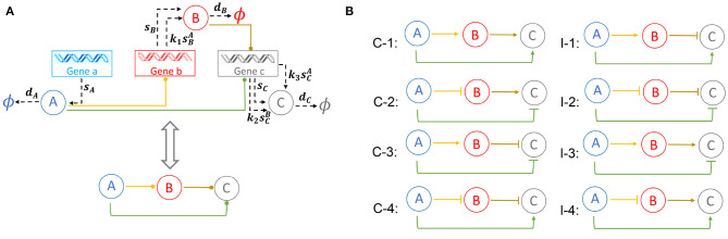
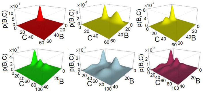
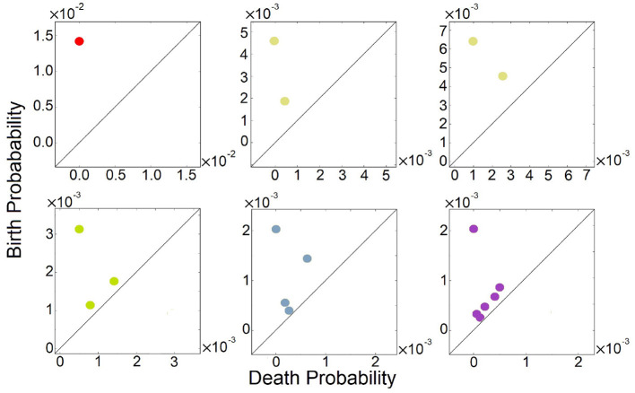
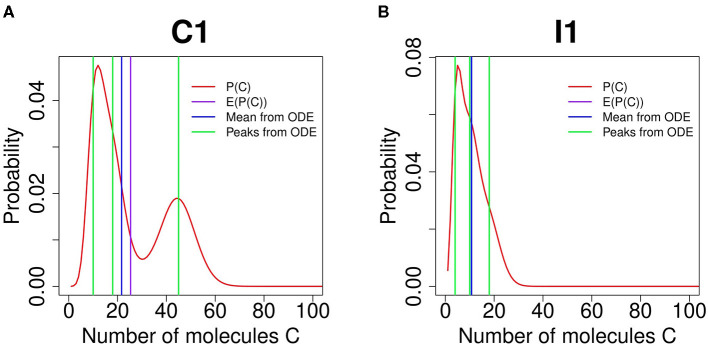
Feed-forward loops (FFLs) are among the most ubiquitously found motifs of reaction networks in nature. However, little is known about their stochastic behavior and the variety of network phenotypes they can exhibit. In this study, we provide full characterizations of the properties of stochastic multimodality of FFLs, and how switching between different network phenotypes are controlled. We have computed the exact steady-state probability landscapes of all eight types of coherent and incoherent FFLs using the finite-butter Accurate Chemical Master Equation (ACME) algorithm, and quantified the exact topological features of their high-dimensional probability landscapes using persistent homology. Through analysis of the degree of multimodality for each of a set of 10,812 probability landscapes, where each landscape resides over 105-106 microstates, we have constructed comprehensive phase diagrams of all relevant behavior of FFL multimodality over broad ranges of input and regulation intensities, as well as different regimes of promoter binding dynamics. In addition, we have quantified the topological sensitivity of the multimodality of the landscapes to regulation intensities. Our results show that with slow binding and unbinding dynamics of transcription factor to promoter, FFLs exhibit strong stochastic behavior that is very different from what would be inferred from deterministic models. In addition, input intensity play major roles in the phenotypes of FFLs: At weak input intensity, FFL exhibit monomodality, but strong input intensity may result in up to 6 stable phenotypes. Furthermore, we found that gene duplication can enlarge stable regions of specific multimodalities and enrich the phenotypic diversity of FFL networks, providing means for cells toward better adaptation to changing environment. Our results are directly applicable to analysis of behavior of FFLs in biological processes such as stem cell differentiation and for design of synthetic networks when certain phenotypic behavior is desired.

Keywords: ACME algorithm; feed forward loop; gene regulatory network; network motif; persistent homology; stochastic reaction network; systems biology.


Conflict of interest statement

YC was employed by company Merck & Co., Inc., Kenilworth, NJ, United States. The remaining authors declare that the research was conducted in the absence of any commercial or financial relationships that could be construed as a potential conflict of interest.

Figures

Figure 1
Figure 1
Representation and the types of feed-forward loop (FFL) network: (A) General wiring and corresponding 3-node schematic representation of an FFL module containing three genes a, b, and c expressing three proteins A, B, and C. Protein A regulates the expressions of genes b and c through binding to their promoters. Protein B regulates the expression of gene c through promoter binding. (B) The FFL modules can be classified into eight different types. Coherent/incoherent FFLs are on the left/right, respectively.
Figure 2
Figure 2
Examples of multimodality exhibited by feed-forward loop (FFL) network motifs. The steady-state probability landscape can exhibit up to 6 different multimodes. The illustrative examples are as follows: 1 peak (red), coherent FFL of type C1 when k1 = 1.2, k2 = 1.2, and k3 = 1.2; 2 peaks (yellow), either in protein B with coherent FFL of type C1, where k1 = 3.0, k2 = 1.2, and k3 = 1.2, or in protein C with coherent FFL of type C1, where k1 = 1.2, k2 = 6.0, and k3 = 6.0; 3 peaks (green), coherent FFL of type C1, where k1 = 1.2, k2 = 6.0, and k3 = 3.6; 4 peaks (light-blue), coherent FFL of type C1 exhibits two peaks for protein B and two peaks for protein C, where k1 = 3.0, k2 = 6.0, and k3 = 6.0; and 6 peaks (purple), coherent FFL of type C1 exhibit two peaks for B and three peaks for C, where k1 = 3.0, k2 = 6.0, and k3 = 3.6.
Figure 3
Figure 3
Persistent diagrams (PDs) of feed-forward loop (FFL) network modules of Figure 2 exhibiting different multimodalities. Red: The probability landscape with monomodality. Yellow: These two PDs depict the two steady-state landscapes exhibiting bimodality. Green, light blue, and purple: These three PDs depict the landscape exhibiting tri-modality, 4-modality, and 6-modality, respectively.
Figure 4
Figure 4
Comparing feed-forward loop (FFL) behavior by Accurate Chemical Master Equation (ACME) and by deterministic ordinary differential equation (ODE) models. (A) shows the results of FFL of C1 type for (k1, k2, k3) = (2.4, 4.5, 1.8). The exact results obtained using ACME exhibit bimodality in protein C (red curve), while trimodality is predicted by the deterministic ODE model (green vertical lines). The mean copy number from ACME (purple vertical line) is also different from the that from ODE (blue vertical line). (B) shows the results of FFL of I1 type for (k1, k2, k3) = (2.4, 0.4, 1.8). The exact results obtained using ACME exhibit monomodality in protein C (red curve), while deterministic ODE model predicts trimodality (green vertical lines), even though the mean copy number of protein C are the same between ACME and ODE models (purple and blue vertical lines, respectively).
Figure 5
Figure 5
Comparing landscapes from Accurate Chemical Master Equation (ACME) and reaction trajectories from the stochastic simulation algorithm (SSA). (A) Probability surface projected onto the (B, C)-plane for the feed-forward loop (FFL) with (k1, k2, k3) = (3.0, 0.5, 5.0). There is bimodality in both proteins B and C. (B,C) The reaction trajectories computed from SSA corresponding to condition in (A) for proteins C and B, respectively. The upper plots are for 2,500 s and lower plots are for 5,000 s. SSA does not capture the bimodality of proteins B and C until 2,500 s. (D) The probability surface projected onto (BC) plain for FFL with (k1, k2, k3) = (0.1, 2.75, 5.0). There is tri-modality in protein C and bimodality in protein B. (E,F) Corresponding reaction trajectories in proteins C and B, respectively. Upper plots are for the results for 2,500 s and lower plots are for 5,000 s. SSA does not capture tri-modality of protein C until 2,500 s. In addition, SSA fails to capture bimodality in protein B.
Figure 6
Figure 6
Phase diagrams of multimodality of Feed-forward loop (FFL) network modules based on 10,812 steady-state probability landscapes at different condition of regulation intensities for all 8 types of FFL network modules. Monomodality occurs when 0.4 ≤ k1 ≤ 2.1 and k2, k3 intensities are moderate, i.e., 0.4 ≤ k1 ≤ 3 (blue region when k1 = 0.4, 0.8, 1.5, and 2.1). Bimodality may occur for different combinations of regulation intensities. When k1 intensity is either very high (2.4 ≤ k1) or very low (k1 ≤ 0.1), bimodality occurs when k2, k3 intensities are moderate, i.e., 0.4 ≤ k1 ≤ 3. When k1 intensity is moderate (0.4 ≤ k1 ≤ 2.1), bimodality occurs when at least one of the other regulation intensities k2 or k3 is high. Tri-modality occurs when k1 is moderate (0.4 ≤ k1 ≤ 2.1) and either k2 or k3 is moderate. Multimodality occurs when k1 is low or high (k1 ≤ 0.4 or k1 ≥ 2.1), and at least either k2 or k3 is high. Color scheme (vertical bar): Blue, green, red, orange, purple, and brow represent regions with one, two three, four, five, and six peaks, respectively.
Figure 7
Figure 7
Effects of input intensity on multimodality of Feed-forward loops (FFLs). The phase diagrams of the number of stability peaks in the steady-state probability landscapes at strong input intensity sA = 10.0 (top row) and weak input intensity sA = 3.0 (bottom row) for different k2 and k3 at three different conditions of k1 = 0.8, 2.1, and 2.4. Color scheme (vertical bar): Blue, green, red, orange, purple, and brown represent regions with one, two, three, four, five, and six peaks, respectively.
Figure 8
Figure 8
Effect of binding dynamics on the modality of protein C in the feed-forward loop (FFL) network of type I1, with (k1, k2, k3) = (3.0, 0.025, 5.1). (A) Effects when binding affinity between gene c and both protein A and protein B are altered by n-fold, where n ∈ {0.5, 2, 8, 16}. At slower binding (yellow line), the modes of distribution of protein C are well-distinguished. However, when the binding and unbinding rates increased to 8 (green line), the peak at C = 9 disappears. At n = 16, bimodality is observed in protein C. (B) Effects when only the binding affinity of gene c and protein B is altered by n-fold, where n ∈ {0.5, 2, 8, 16}. When the binding affinity of gen c and protein B increases, the peak at C = 9 disappears, while the peaks at C = 49 robustly remains. However, the peak at C = 49 becomes less significant. (C) Effects when only the binding affinity of gen c and protein A is altered by n-fold, where n ∈ {0.5, 2, 8, 16}. At high binding affinity, the peak at C = 9 disappears while the peak at C = 49 becomes more prominent.
Figure 9
Figure 9
Phase diagram of the effects of gene duplication on multimodality of feed-forward loops (FFLs). First row: Phase diagrams of the modality of stability peaks when there are one copy of gene c and one copy of gene b. Second row: Phase diagrams when there are one copy of gene b and two copies of gene c. Third row: Phase diagram, when there are two copy of gene b and one copy of gene c. The first, second, and third columns are for k1 = 0.025, 1.5, and 2.4, respectively. Color scheme (vertical bar): Blue, green, red, orange, purple, and brown represent regions with one, two, three, four, five, and six peaks, respectively.

Similar articles

Cited by

References

    1. Acar M., Becskei A., van Oudenaarden A. (2005). Enhancement of cellular memory by reducing stochastic transitions. Nature 435, 228–232. 10.1038/nature03524 - DOI - PubMed
    1. Ali Al-Radhawi M., Del Vecchio D., Sontag E. D. (2019). Multi-modality in gene regulatory networks with slow promoter kinetics. PLoS Comput. Biol. 15:e1006784. 10.1371/journal.pcbi.1006784 - DOI - PMC - PubMed
    1. Alon U. (2006). An Introduction to Systems Biology: Design Principles of Biological Circuits. New York, NY: CRC Press. 10.1201/9781420011432 - DOI
    1. Arkin A., Ross J., McAdams H. H. (1998). Stochastic kinetic analysis of developmental pathway bifurcation in phage λ-infected Escherichia coli cells. Genetics 149, 1633–1648. 10.1093/genetics/149.4.1633 - DOI - PMC - PubMed
    1. Boyer L. A., Lee T. I., Cole M. F., Johnstone S. E., Levine S. S., Zucker J. P., et al. . (2005). Core transcriptional regulatory circuitry in human embryonic stem cells. Cell 122, 947–956. 10.1016/j.cell.2005.08.020 - DOI - PMC - PubMed

LinkOut - more resources