Decoding locomotion from population neural activity in moving C. elegans

Abstract

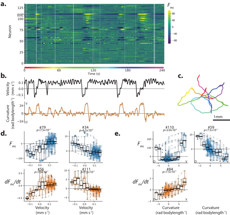
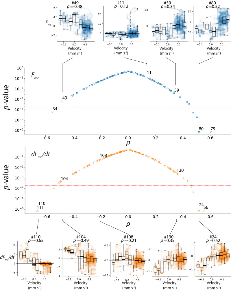
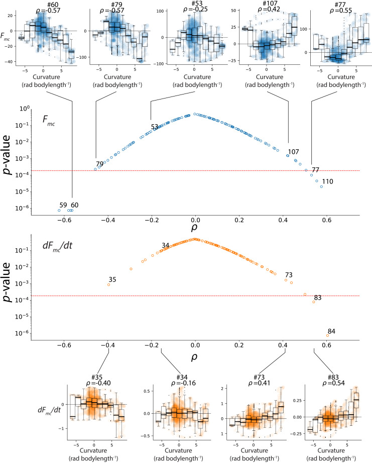
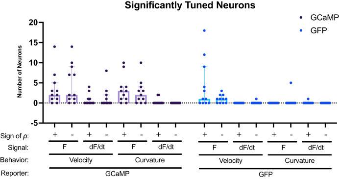
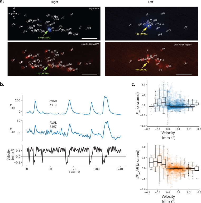
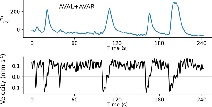
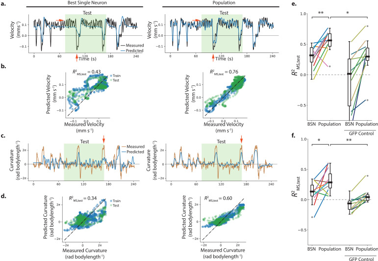
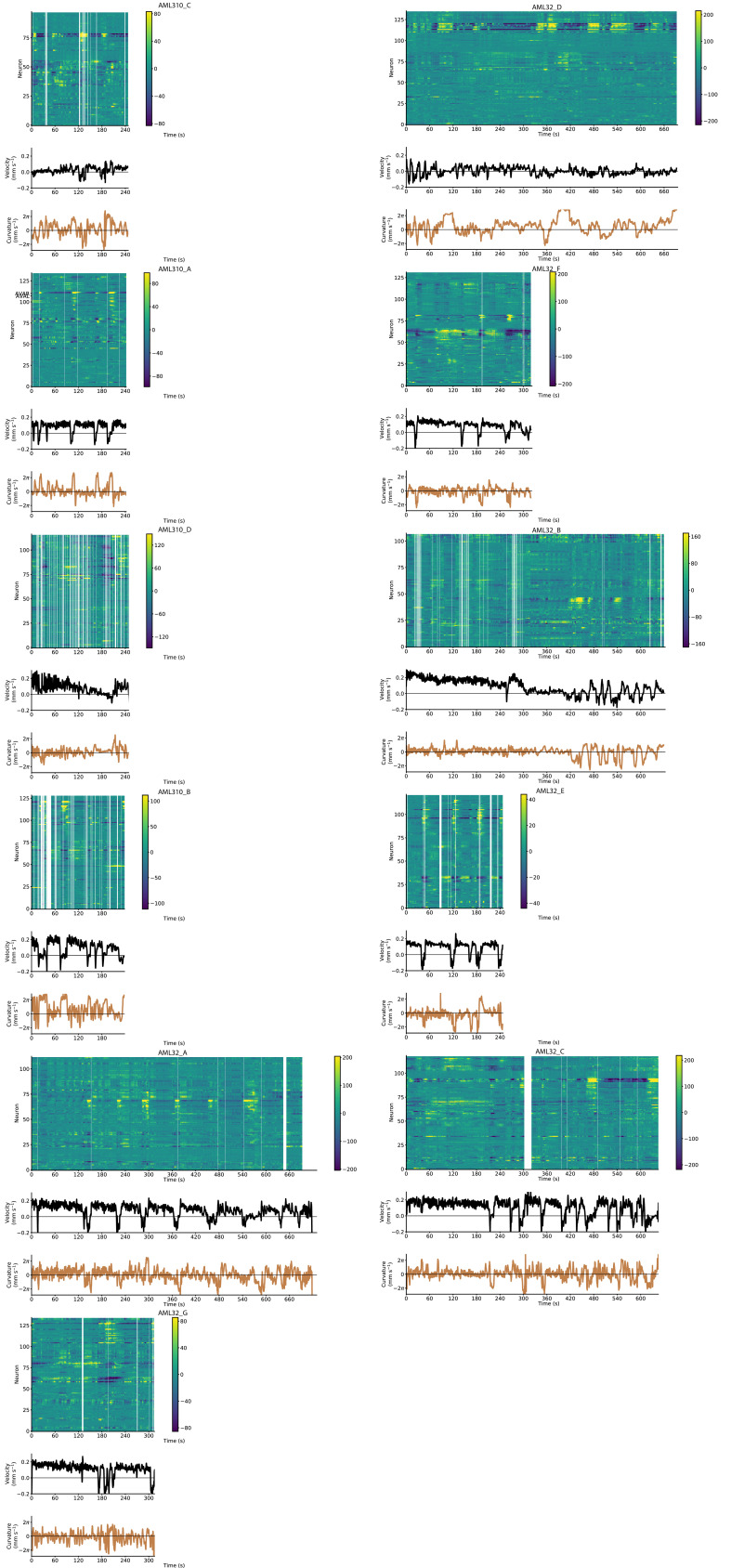
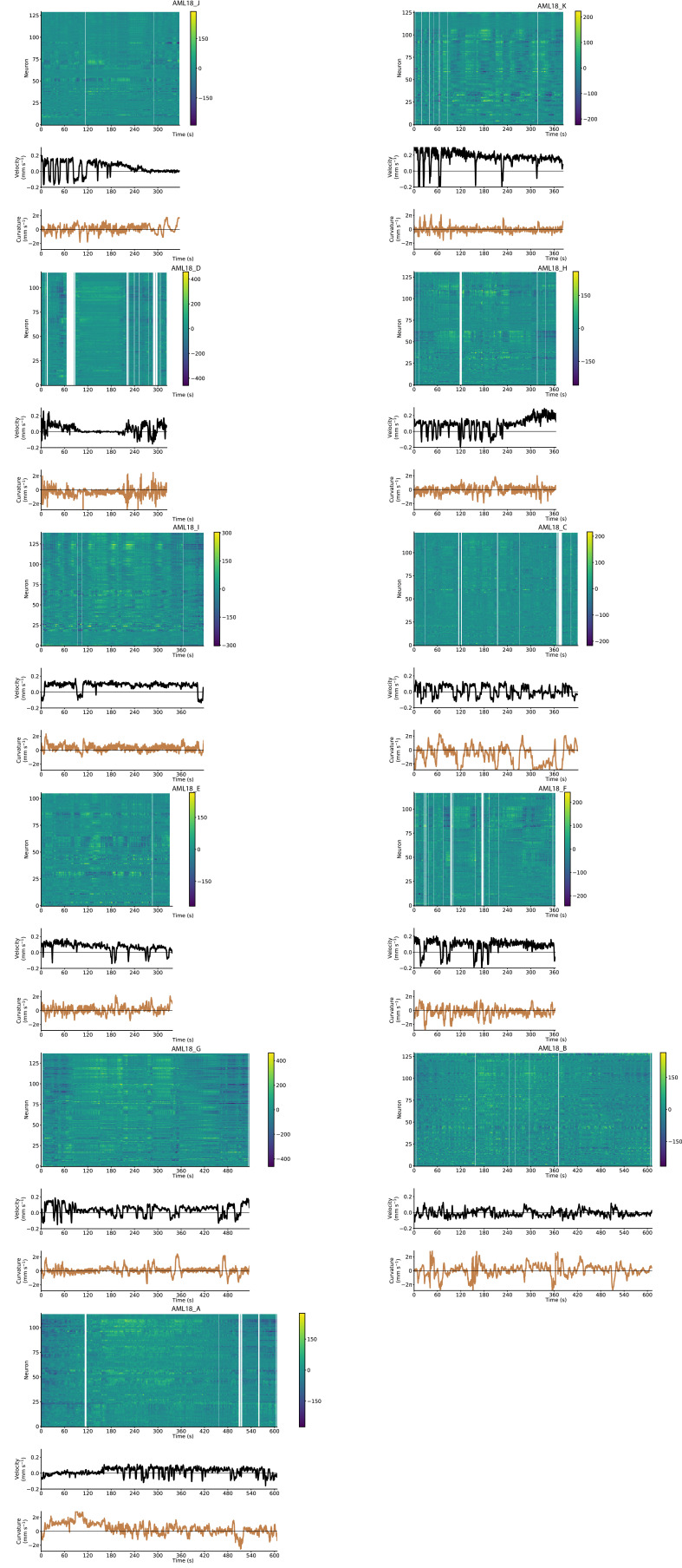
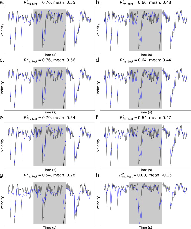
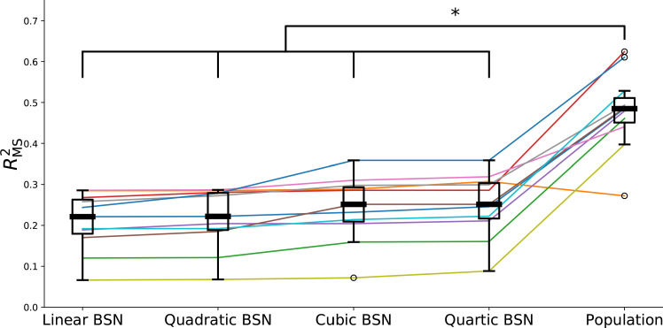
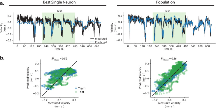
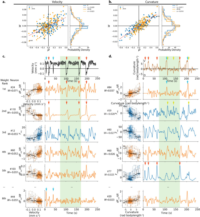
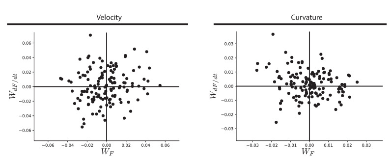
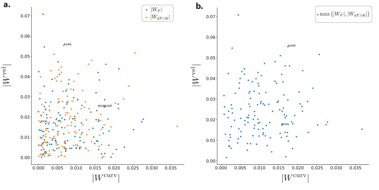
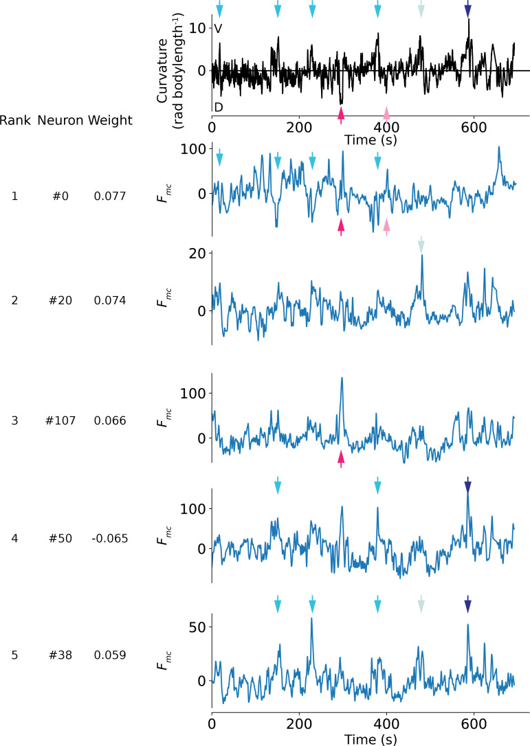
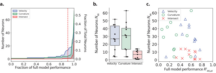
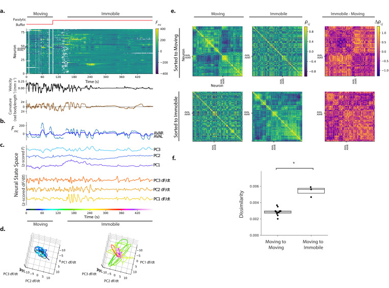
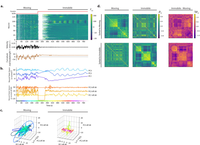
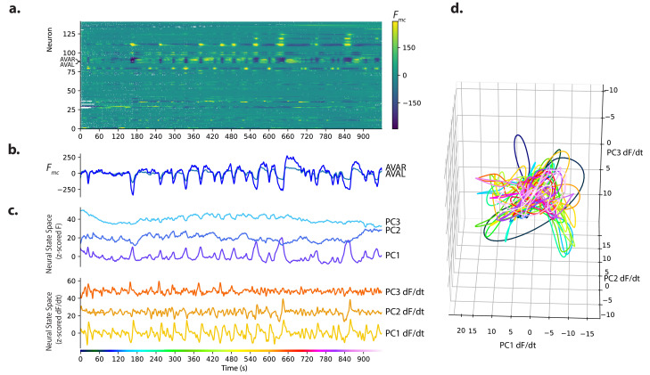
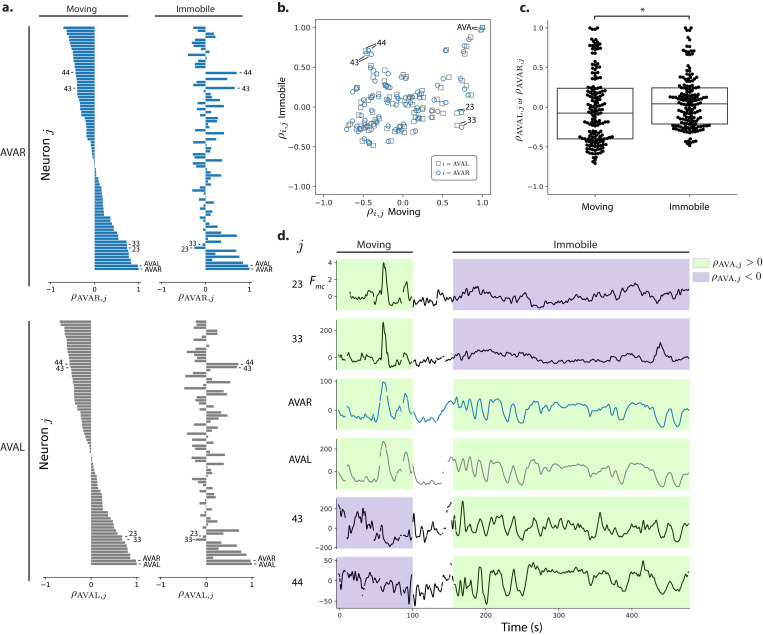
We investigated the neural representation of locomotion in the nematode C. elegans by recording population calcium activity during movement. We report that population activity more accurately decodes locomotion than any single neuron. Relevant signals are distributed across neurons with diverse tunings to locomotion. Two largely distinct subpopulations are informative for decoding velocity and curvature, and different neurons' activities contribute features relevant for different aspects of a behavior or different instances of a behavioral motif. To validate our measurements, we labeled neurons AVAL and AVAR and found that their activity exhibited expected transients during backward locomotion. Finally, we compared population activity during movement and immobilization. Immobilization alters the correlation structure of neural activity and its dynamics. Some neurons positively correlated with AVA during movement become negatively correlated during immobilization and vice versa. This work provides needed experimental measurements that inform and constrain ongoing efforts to understand population dynamics underlying locomotion in C. elegans.

Keywords: C. elegans; behavior; calcium imaging; decoding; locomotion; neural dynamics; neuroscience; physics of living systems; population code.

Figure 1.. Population calcium activity and tuning of select neurons during spontaneous animal movement.

Recording AML310_A. (a) Calcium activity of 134 neurons is simultaneously recorded during locomotion. Activity is displayed as motion-corrected fluorescent intensity $F_{mc}$. Neurons are numbered according to agglomerative hierarchical clustering. White space indicates time-points where neural tracking failed. (b) Body bend velocity and body curvature derived from an eigenvalue decomposition, and (c) position on the plate during recording are shown. (d) Example neurons significantly tuned to velocity. Examples are those with the highest Pearson’s correlation coefficient in each category: activity (or its derivative) with positive (or negative) correlation to velocity. P-values are derived from a shuffling procedure that preserves per-neuron correlation structure. All tuning curves shown are significant at 0.05% after Bonferroni correction for multiple hypothesis testing ($p<1.9\times {10}^{-4}$). Boxplot shows median and interquartile range. Blue or orange shaded circles show neural activity at each time point during behavior. (e) Example neurons highly tuned to curvature were selected similarly. No neurons with negative $dF/dt$ tuning to curvature passed our significance threshold.

Figure 1—figure supplement 1.. Additional details and examples of velocity tuning.

Additional examples of velocity tuning curves for $F_{\text{mc}}$ (top) and $d{F}_{\text{mc}}/dt$ (bottom) from recording AML310_A are shown. The correlation coefficient ρ captures the relation between each neuron’s activity and curvature and is plotted with a corresponding p-value (middle). The p-value is calculated from a time-lag shuffle and tests the null hypothesis that such a correlation would be found due to chance. Dashed line indicates a significance level of 0.05 after a Bonferonni correction for multiple hypothesis testing ($p<1.9\times {10}^{-4}$).

Figure 1—figure supplement 2.. Additional details and examples of curvature tuning.

Additional examples of curvature tuning for $F_{\text{mc}}$ (top) and $d{F}_{\text{mc}}/dt$ (bottom) from recording AML310_A are shown. The correlation coefficient ρ captures the relation between each neuron’s activity and velocity and is plotted with a corresponding p-value (middle). The p-value is calculated from a time-lag shuffle and tests the null hypothesis that such a correlation would be found due to chance. Dashed line indicates a significance level of 0.05 after a Bonferonni correction for multiple hypothesis test ($p<1.9\times {10}^{-4}$).

Figure 1—figure supplement 3.. Number of significantly tuned neurons across recordings.

Pearson’s correlation coefficient ρ was calculated for each neuron in 11 GCaMP recordings and 11 GFP control recordings that lacked a calcium indicator. Neurons were counted as significantly tuned if their Pearson’s correlation coefficient passed a recording-specific multiple-hypothesis corrected significance test and exceeded an absolute value of 0.4. Bar shows median. Whiskers show inter-quartile range.

Figure 2.. Neuron pair AVA is active during backward locomotion and exhibits expected tuning during moving population recordings.

(a) AVAR and AVAL are labeled by BFP under a rig-3 promoter in strain AML310. Two optical planes are shown from a single volume recorded during movement. Planes are near the top and bottom of the optical stack, corresponding to the animals’ extreme right and left. The recording is the same as in Figure 1. Top row shows BFP. Bottom row shows RFP in the nuclei of all neurons. Segmented neurons centered in the optical plane are labeled with ⊕, while neurons from nearby optical planes are labeled with ○. Arrow indicates AVAR or AVAL. Numbering corresponds to Figure 1a. (b) Calcium activity of AVAR and AVAL during locomotion in recording AML310_A, same as in Figure 1. (c) Aggregate tuning of AVA across four individuals (seven neurons). Boxplot shows median and interquartile range. Lightly shaded blue or orange circles show activity at each time point during behavior.

Figure 2—figure supplement 1.. Sum of AVAL and AVAR activity.

Activity of AVAL and AVAR from AML310_A in Figure 2b are shown summed together. This permits comparison to recordings that do not resolve the two neurons separately.

Figure 3.. Population neural activity decodes locomotion.

(a–d) Performance of the best single neuron (BSN) is compared to a linear population model in decoding velocity and body curvature for the exemplar recording AML310_A shown in Figure 1. (a) Predictions on the held-out test set are compared to measured velocity. Light green shaded region indicates held-out test set. Red arrows indicate examples of features that the population captures better than the BSN. (b) Performance is reported as a coefficient of determination $R_{\mathrm{MS}}^2$ evaluated on the mean-subtracted held-out test data (green points). (c,d) Model predictions are compared to measured curvature. (e) Performance of velocity decoding is shown for recordings of $n=11$ individuals (strain AML310 and AML32) and for recordings of $n=11$ GFP control animals lacking a calcium indicator (strain AML18). Two-sided Wilcoxon rank test is used to test significance of population performance compared to BSN, ${\displaystyle p=3.9\times {10}^{-3}}$. Welch’s unequal variance t-test is used to test significance of population performance compared to GFP control, $p=3.2\times {10}^{-2}$. (f) Performance of curvature decoding is shown for all recordings. Each recording is colored the same as in e. $p=3.2\times {10}^{-2}$ and $p=1.8\times {10}^{-3}$ for comparisons of population performance to that of BSN, and GFP control, respectively.

Figure 3—figure supplement 1.. Performance correlates with maximal GCaMP Fano Factor, a metric of signal.

Decoding performance is plotted against maximal GCaMP Fano Factor for each recording for velocity and curvature. Maximal GCaMP Fano Factor is the Fano Factor of the raw GCaMP activity for the neuron in each recording with the highest Fano Factor, ${\max }_i\left(\frac{{\sigma }^2[F_{i,\mathrm{GCaMP}}]}{\mu [F_{i,\mathrm{GCaMP}}]}\right)$. Labels for each recording are shown. Dashed red line is the line of best fit (correlation coefficient between fit and data is $\rho =0.46$ for velocity and $\rho =0.49$ for curvature).

Figure 3—figure supplement 2.. Neural activity and behavior for all moving calcium imaging recordings (AML310 and AML32).

Figure 3—figure supplement 3.. Neural activity and behavior for all moving GFP control recordings (AML18).

Neural activity and behavior for all moving GFP control recordings (AML18).

Figure 3—figure supplement 4.. Alternative population models.

Performance of alternative population models for decoding velocity. Traces are shown for exemplar recording AML310_A. Mean across all moving GCaMP recordings is also listed. Gray shading shows held-out test set. (a) The population model used throughout the paper. This model uses ridge regression with fluorescence signals and their temporal derivatives as features. (b) A linear model using ridge regression, with only fluorescence (not temporal derivative) signals as features. (c) A linear model using fluorescence signals and their temporal derivatives as features, regularized with a combination of a ridge penalty and the squared error of the temporal derivative of behavior. (d) The model in c, but using only fluorescence signals as features. (e) A linear model using fluorescence signals and their temporal derivatives as features, regularized with an ElasticNet penalty with an L₁ ratio of ${10}^{-2}$. (f) The model in e, but using only fluorescence signals as features. (g) The multivariate adaptive regression splines (MARS) model, using fluorescence signals and their temporal derivatives as features. (h) A linear model together with a shallow decision tree, using fluorescence signals and their temporal derivative as features.

Figure 3—figure supplement 5.. Nonlinear fits using best single neuron.

Performance of polynomial regression models for decoding velocity on 11 GCaMP recordings using the best single neuron. The best single neuron is defined as the one with the best decoding performance using a linear model on the training data. We compare the performance of these regression models to that of the population model using a two-sided Wilcoxon rank test. The population model significantly (p < 0.05) outperforms polynomial regression models up to fourth order.

Figure 4.. Example where population decoded a fuller range of animal behavior.

(a) The decoding from the best single neuron and the population model are compared to the measured velocity for example recording AML32_A. (b) Predictions from the best single neuron saturate at a velocity of approximately 0.1 mm s⁻¹.

Figure 5.. Weights assigned to neurons by the population model in the exemplar recording, and their respective tuning.

(a) The weight $W$ assigned to each neuron’s activity ($F_{\text{mc}}$) or its temporal derivative ($d{F}_{\text{mc}}/dt$) by the velocity population decoder is plotted against its Pearson’s Correlation coefficient ρ which characterizes its tuning to velocity. Recording AML310_A is shown, same as in Figure 1. Dashed red line shows line of best fit. Right panel shows the observed distribution of weights. A zero-mean Gaussian with standard deviation set to the empirically observed standard deviation is also shown. (b) Same as in a, but for curvature. (c) Tuning and activity of the top highest amplitude weighted neurons for velocity is shown. Activity of each neuron is time aligned to the observed behavior (top row). Neurons are labeled corresponding to their number in the heatmap in Figure 1. Their rank and weight $W$ in the decoder is listed. Red arrows highlight peaks in the temporal derivative of activity of neuron #24 and #110, while cyan arrows highlight peaks of neuron #44. Y- and X-axes labels and scales are preserved within individual rows and columns, respectively. Light green shading indicates the held-out portion of the recording. (d) Same as c but for curvature. Red and cyan arrows show two sets of deep ventral bends that are captured by different neurons. Green arrows show dorsal bends.

Figure 5—figure supplement 1.. Comparison of weights assigned to a neuron’s activity versus its temporal derivative.

Comparison of weights assigned to a neuron’s activity versus its temporal derivative for velocity (left) or curvature (right) decoders. Comparison of weights assigned to a neuron’s activity $|W_F|$ by the population decoder, versus the weights assigned to its temporal derivative $|W_{dF/dt}|$ for each neuron in recording AML310_A.

Figure 5—figure supplement 2.. Comparison of weights assigned for decoding velocity vs decoding curvature.

Comparison of weights assigned for decoding velocity vs decoding curvature. (a) The magnitude of the weight assigned to each neuron in recording AML310_A for velocity $|W^{\mathrm{vel}}|$ is compared to the magnitude of its assigned weight for curvature $|W^{\mathrm{curv}}|$. Each neuron is plotted twice, once for the weight assigned to its activity and once for the weight assigned to the temporal derivative of its activity. (b) Same as in (a), except here the higher weight of either activity or its temporal derivative is plotted.

Figure 5—figure supplement 3.. Example traces of highly weighted neurons used to decode curvature in AML32_A.

Traces of top five highest weighted neurons used to decode curvature in AML32_A. Same recording as in Figure 4. Arrows indicate activity peaks corresponding to ventral (blue shades, top) or dorsal turns (red shades, bottom). Different neurons contribute activity peaks to different sets of turns.

Figure 6.. Number of neurons needed by the model to decode velocity and curvature.

(a) The minimum number of neurons needed for a restricted model to first achieve a given performance is plotted from recording AML310_A in Figure 1. Performance, $R_{\text{MS,all}}^2$ is reported separately for velocity (blue) and curvature (green) and is calculated on the entire recording (test and train). Intersect refers to the intersection of the set of neurons included in both partial models (velocity and curvature) for a given performance. Red dashed line, N₉₀, indicates number of neurons needed to achieve 90% of full model performance. (b) N₉₀ is computed for velocity and curvature for all recordings. The number of neurons present in both populations at 90% performance level (intersection) is shown. Box shows median and interquartile range. (c) N₉₀ for all recordings is shown plotted versus the performance of the full population velocity or curvature decoder, respectively. Number of intersection neurons (red ’x’) is plotted at the higher of either the velocitys or curvature’s performance.

Figure 7.. Immobilization alters the correlation structure of neural activity.

(a) Calcium activity is recorded from an animal as it moves and then is immobilized with a paralytic drug, recording AML310_E. (b) Activity of AVAL and AVAR from (a). (c) Population activity (or its temporal derivative) from (a) is shown projected onto its first three PCs, as determined by only the immobilized portion of the recording. (d) Neural state space trajectories from (c) are shown split into moving and immobile portions, color coded by time. Scale, axes and PCs are the same in both plots. (e) Pairwise correlations of neural activity ${\rho }_{i,j}$ are shown as heatmaps for all neurons during movement and immobilization, sorted via a clustering algorithm. Top row is sorted to movement, bottom row is sorted to immobilization. (f) Dissimilarity between correlation matrices for moving and immobile portions of a recording are shown compared to the dissimilarity observed between correlation matrices taken at similar time windows within moving-only recordings. Dissimilarity is $\sqrt{⟨{({\rho }_{i,j}^{\prime }-{\rho }_{i,j})}^2⟩}$. Dissimilarity was measured in three moving-immobile recordings with paralytic and 11 moving-only recordings. ${\displaystyle p=1.2\times {10}^{-2}}$, Welch’s unequal variance t-test. Boxes show median and interquartile range.

Figure 7—figure supplement 1.. Example from additional moving-to-immobile recording.

Calcium activity is recorded from an animal as it moves and then is immobilized with a paralytic drug, recording AML32_H. Activity and behavior. (b) Population activity (or its derivative) from (a) is shown projected onto its first three PCs, as determined by only the immobilized portion of the recording. (c) Neural state space trajectories from (b) are plotted in 3D and shown split into moving and immobile portions. (d) Pairwise correlations of neural activity ${\rho }_{i,j}$ are shown as heatmaps for all neurons during movement and immobilization, sorted via clustering algorithm. Top and bottom rows are sorted to movement or immobilization, respectively.

Figure 7—figure supplement 2.. Immobile-only recording.

Calcium activity is recorded from an animal immobilized with nano-beads, recording AML310_G. (a) Calcium activity. (b) Activity of neurons AVAL and AVAR. (c) Population activity (or its temporal derivative) from (a) is shown projected onto its first three PCs, as determined by only the immobilized portion of the recording. (d) Neural state space trajectories from (b) are plotted in 3D.

Figure 8.. Correlations with respect to AVAL and AVAR during movement and immobilization.

(a) The Pearson’s correlation of each neuron’s activity to AVAR and AVAL is shown during movement and immobilization. Selected neurons are numbered as in Figure 7 (same recording, AML310_E). Neurons are sorted according to their correlation during movement. (b) Scatter plot shows relation between a neuron’s correlation to AVA during movement and its correlation during immobilization. Gray squares and blue circles indicate correlation to AVAL and AVAR, respectively. (c) On average, neurons become more positively correlated to AVA upon immobilization, p = 0.019 Wilcoxon ranked test. Box shows median and interquartile range. (d) Activity traces of selected neurons are shown time aligned to AVA. Green and purple shading indicate positive or negative correlation to AVA, respectively.

References

1. Ahrens MB, Li JM, Orger MB, Robson DN, Schier AF, Engert F, Portugues R. Brain-wide neuronal dynamics during motor adaptation in zebrafish. Nature. 2012;485:471–477. doi: 10.1038/nature11057. - DOI - PMC - PubMed
1. Ben Arous J, Tanizawa Y, Rabinowitch I, Chatenay D, Schafer WR. Automated imaging of neuronal activity in freely behaving Caenorhabditis elegans. Journal of Neuroscience Methods. 2010;187:229–234. doi: 10.1016/j.jneumeth.2010.01.011. - DOI - PubMed
1. Berman GJ, Bialek W, Shaevitz JW. Predictability and hierarchy in Drosophila behavior. PNAS. 2016;113:11943–11948. doi: 10.1073/pnas.1607601113. - DOI - PMC - PubMed
1. Brennan C, Proekt A. A quantitative model of conserved macroscopic dynamics predicts future motor commands. eLife. 2019;8:e46814. doi: 10.7554/eLife.46814. - DOI - PMC - PubMed
1. Briggman KL, Abarbanel HD, Kristan WB. Optical imaging of neuronal populations during decision-making. Science. 2005;307:896–901. doi: 10.1126/science.1103736. - DOI - PubMed
Publication types