State-Of-The-Art Quantification of Polymer Solution Viscosity for Plastic Waste Recycling

Abstract

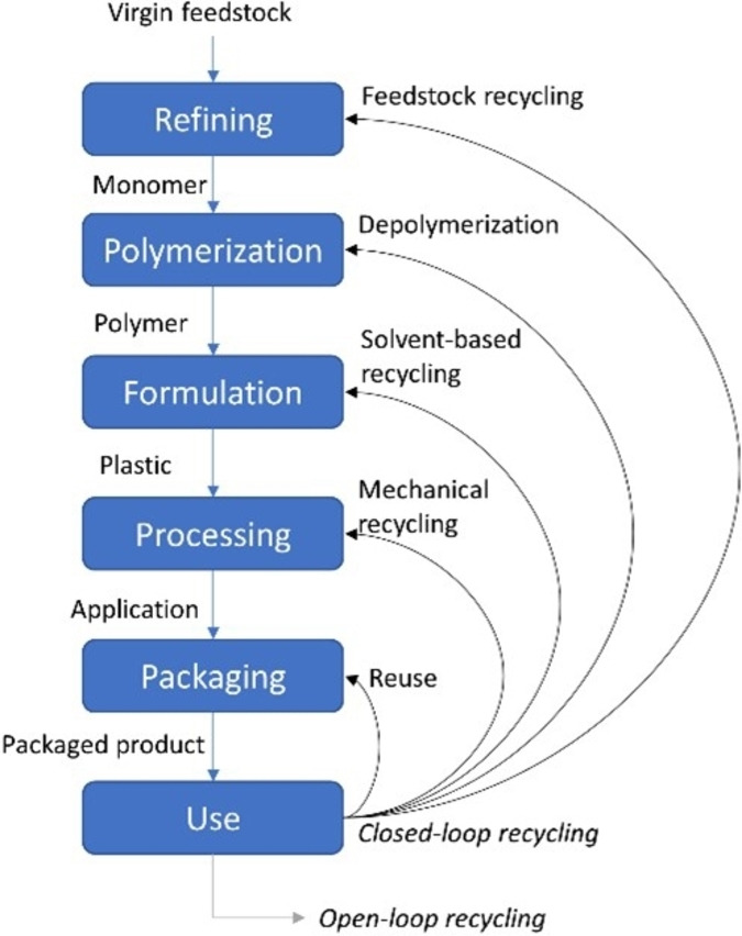
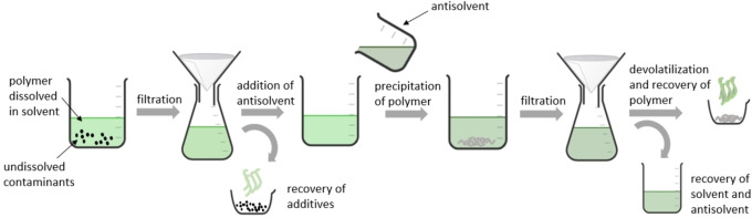
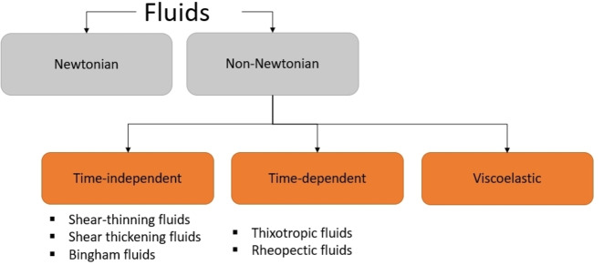
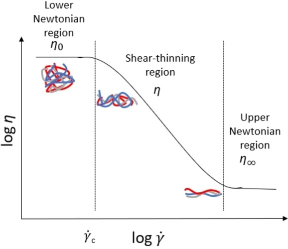
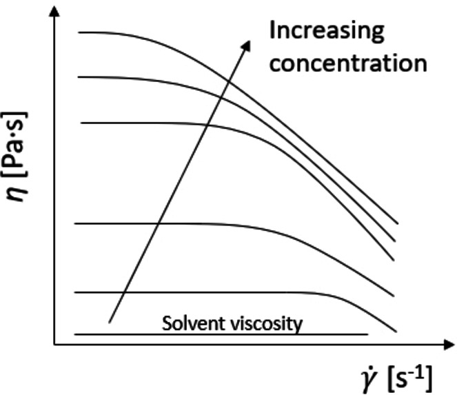
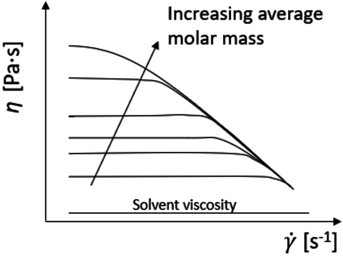
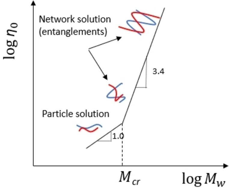
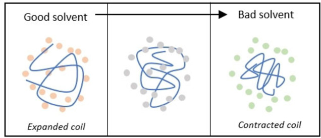
Solvent-based recycling is a promising approach for closed-loop recovery of plastic-containing waste. It avoids the energy cost to depolymerize the plastic but still allows to clean the polymer of contaminants and additives. However, viscosity plays an important role in handling the polymer solutions at high concentrations and in the cleaning steps. This Review addresses the viscosity behavior of polymer solutions, available data, and (mostly algebraic) models developed. The non-Newtonian viscosity models, such as the Carreau and Yasuda-Cohen-Armstrong models, pragmatically describe the viscosity of polymer solutions at different concentrations and shear rate ranges. This Review also describes how viscosity influences filtration and centrifugation processes, which are crucial steps in the cleaning of the polymer and includes a polystyrene/styrene case study.

Keywords: dyes/pigments; plastics recycling; separations; solvent effects; viscosity.

Figure 1

Positioning of solvent‐based recycling. Figure adapted from ref. [10].

Figure 2

Dissolution−precipitation process. Figure adapted from ref. [1].

Figure 3

Newtonian and non‐Newtonian fluids.

Figure 4

Log–log relationship between viscosity and shear rate for polymer solutions and melts. Figure adapted with permission from ref. [31]; copyright John Wiley and Sons, 2018 and from ref. [37]; copyright Carl Hanser Verlag, 2015. [ ³¹ , ³⁷ , ³⁸ , ⁴⁰ ]

Figure 5

Schematic representation of system in which (a) We≪1, where polymer chains are weakly perturbed, close to their equilibrium conformation and (b) We≫1 in which the polymers are subject to considerable stretching and there is a clear influence of flow. Orange lines represent highlighted polymer chains. Adapted with permission from ref. [54]; copyright American Chemical Society, 2010.

Figure 6

Influence of polymer solution concentration on the viscosity behavior. Figure adapted with permission from ref. [27] for polystyrene in toluene at different concentrations and fixed average molar mass; copyright Springer Nature, 1984.

Figure 7

Influence of the average molar mass on the viscosity behavior. Figure adapted with permission from ref. [27] for PS/toluene solution at different molar masses and a fixed concentration; copyright Springer Nature, 1984.

Figure 8

Typical 3.4 power law behavior of highly concentrated polymer solutions and melts. The blue and red lines represent polymer chains. Figure adapted with permission from ref. [29]; Copyright Springer, 2000 and ref. [37]; Copyright Carl Hanser Verlag, 2015.

Figure 9

The influence of the solvation capacity on the polymer coil dimensions. Blue lines represent the polymer chain, orange, gray and green dots represent different solvents with descending solvent power. Figure adapted from refs. [38] and [78].

Figure 10

Overview of viscosity models for polymer solutions.

Figure 11

Viscous flow according to Eyring: (a) Activation of state. Adapted with permission from ref. [123]; copyright American Chemical Society, 2006. (b) Jump of molecule. Adapted with permission from ref. [124]; copyright American Chemical Society, 1941.

Figure 12

Regions of the linear viscoelastic behavior of polymer solution. Figure adapted from ref. [38].

Figure 13

Overview of the applicability of the models. Both figures are a representative curve for a polymer solution with a fixed M_w. Abbreviations: Cross=Cross model; CombM=combined power law, Cross and Newtonian model; Carreau=Carreau model; YAC=Yasuda−Armstrong−Cohen model; OWPL=Ostwald–de Waele power law model.

Figure 14

Newtonian models applied to a PS and PVC solution and the respective error calculations: (a) PS/styrene solution; T=30 °C, M_w=160000 g mol⁻¹; experimental data from ref. [133]. (b) PVC/cyclohexanone solution; T=30 °C, M_w=110000 g mol⁻¹; experimental data from ref. [63]. (c) TIC, HYBRID and AARD errors for the different models for the PS solution. The HYBRID values are divided by 100. (d) TIC, HYBRID and AARD errors for the different models for the PVC solution. The HYBRID values are again divided by 10. Abbreviations: NRTL=segment‐based Eyring‐NRTL model; Wilson=segment‐based Eyring‐Wilson model; mNRF=segment‐based modified NRF model; NRF=segment‐based Eyring‐NRF model; PMV=polymer mixture viscosity model.

Figure 15

Non‐Newtonian models applied to a PS/toluene solution: (a) 0.5 wt %; (b) 4 wt %; (c) TIC, HYBRID and AARD for the 0.5 wt % solution; (d) TIC, HYBRID and AARD for the 4 wt % solution. Experimental data are from ref. [27]. The HYBRID values are divided by 1000. Abbreviations: CrossInf=cross model with second Newtonian viscosity parameter incorporated; CombM=combined power law, Cross and Newtonian model; CarreauInf=Carreau model with second Newtonian viscosity parameter incorporated; YACInf=Yasuda−Armstrong−Cohen model with second Newtonian viscosity parameter incorporated; OWPL=Ostwald−de Waele power law model.

Figure 16

Application range of filters and centrifuges for a close up to range of particle sizes of 0.1 and 10 μm. Values ranges correspond to the range of concentration of the feed (data from ref. [174]).

Figure 17

Cake‐filtration setup. Reproduced with permission from ref. [175]; copyright Elsevier 2006.

Figure 18

Incompressible and compressible cake filtration. Reprinted with permission from ref. [183]; copyright Elsevier, 1997.

Figure 19

Influence of the viscosity of a PS/styrene solution on the pressure drop considering Newtonian behavior and cake compressibility for TiO₂. Initial data: c ₁=6.04 wt %, c _m,1=0.32 wt %, η _0,1=1.1×10⁻² Pa s. Interpretation of the figure: For c ₂/c ₁=1 and η _0,2/η _0,1=1, ΔP ₂/ΔP ₁ is 1. When c ₂=3 c _1, the viscosity increases 18 times compared to η _0,1, η _0,2/η _0,1=18, and ΔP ₂ increases by 400 times, ΔP ₂/ΔP ₁=398. The data for this graph are given in Table S6 in the Supporting Information.

Figure 20

(a) Influence of viscosity on the sedimentation velocity. (b) Influence of polymer solution concentration on the flow rate. Data for a PS/styrene solution at 30 °C taken from ref. [133].

References

1. Vollmer I., Jenks M. J. F., Roelands M. C. P., White R. J., van Harmelen T., de Wild P., van der Laan G. P., Meirer F., Keurentjes J. T. F., Weckhuysen B. M., Angew. Chem. Int. Ed. 2020, 59, 15402–15423; - PMC - PubMed
2. Angew. Chem. 2020, 132, 15524–15548.
1. PlasticsEurope, Plastics: the Facts 2019, 2019, https://www.plasticseurope.org/en/resources/market-data.
1. Duan L., D'hooge D. R., Cardon L., Prog. Mater. Sci. 2020, 114, 100617.
1. Luijsterburg B. J., Jobse P. S., Spoelstra A. B., Goossens J. G. P., Waste Manage. 2016, 54, 53–61. - PubMed
1. Ragaert K., Delva L., Van Geem K., Waste Manage. 2017, 69, 24–58. - PubMed
LinkOut - more resources