Mice learn multi-step routes by memorizing subgoal locations

Abstract

The behavioral strategies that mammals use to learn multi-step routes are unknown. In this study, we investigated how mice navigate to shelter in response to threats when the direct path is blocked. Initially, they fled toward the shelter and negotiated obstacles using sensory cues. Within 20 min, they spontaneously adopted a subgoal strategy, initiating escapes by running directly to the obstacle's edge. Mice continued to escape in this manner even after the obstacle had been removed, indicating use of spatial memory. However, standard models of spatial learning-habitual movement repetition and internal map building-did not explain how subgoal memories formed. Instead, mice used a hybrid approach: memorizing salient locations encountered during spontaneous 'practice runs' to the shelter. This strategy was also used during a geometrically identical food-seeking task. These results suggest that subgoal memorization is a fundamental strategy by which rodents learn efficient multi-step routes in new environments.

Extended Data Fig 1

Extended Data Fig 2

Extended Data Fig 3

Extended Data Fig 4

Extended Data Fig 5

Extended Data Fig 6

Extended Data Fig 7

Extended Data Fig 8

Extended Data Fig 9

Extended Data Fig 10

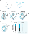
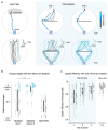
Figure 1. Mice rapidly learn efficient escape trajectories in the presence of obstacles

a, Single escape trials colored by speed (top) and all trajectories color-coded by trajectory type (bottom; homing-vector paths are gray, edge-vector paths are blue). Initial escape target is the direction of the vector from escape initiation to 10 cm in front of the obstacle, normalized between 0 (directed at the shelter) and 1 (directed at the obstacle edge location). Dashed arrows in the top panels illustrate the shelter and edge-vector directions. Dots show the point where the target measurement is taken. Values (0.56 and 1.02) are the escape target score for the examples shown. Dot-and-arrow plots show the distribution of initial escape targets (the arrow is the median value). Only successful escapes (getting to the shelter within 12 seconds) are analyzed. b, Summary of initial escape targets. One-sided permutation test on the target score, trial 1 vs. trials 2-3: P=0.0004 (***). Each dot represents one escape. Gray points are escapes classified as homing vectors and blue points are edge-vector escapes. Differences in escape target were not related to differences in position or angle at the moment of threat onset (Supplementary Fig. 1). c, Spatial efficiency is the ratio of the shortest possible escape path length and the path actually taken to the shelter. This is the inverse of tortuosity. Each dot represents one escape. Open field total: N=23 escapes, 10 mice; obstacle total: N=66 escapes, 24 mice; obstacle trial 1: N=21 escapes, 21 mice; obstacle trial 2: N=24 escapes, 24 mice; obstacle trial 3: N=21 escapes, 21 mice; obstacle trials 2-3: N=45 escapes, 24 mice. White squares show the median, thick lines show the IQR, and thin lines show the range excluding outliers (beyond the median ± 1.5 x IQR). Distributions are kernel density estimates.

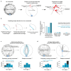
Figure 2. Mice use a spatial memory strategy for efficient obstacle avoidance

a, Examples of edge-vector escape trials (top) and all trajectories (bottom) after removing the obstacle. Subheaders describe the experience in the environment prior to removing the obstacle. The dotted line indicates where the obstacle used to be. Arrow plots show the distribution of initial escape targets. b, Summary data for initial escape targets after obstacle removal. One-sided permutation test: acute: P=1x10^-5 (***); chronic 3 baseline: P=0.02 (*); chronic 0 baseline: P=0.004 (**), permutation test on the rate of edge-vectors compared to the open field. Acute removal: N=8 escapes, 8 mice; chronic removal, 3 baselines: N=18 escapes, 8 mice; chronic removal, 0 baselines: N=23 escapes, 10 mice. c, Schematic for the experiment in which the obstacle length is changed by 25%. For the “obstacle shortened” condition, the dotted gray line indicates the initial obstacle length, and the thick black line indicates the new length (after 20 minutes / 3 baseline escape trials). For the “obstacle lengthened” condition, the thick black line indicates the initial obstacle length, and the dotted gray line indicates the new length. Both the initial and the shelter-bound segments of the escape are analyzed. d, Summary data for the experiments changing the length of the obstacle by 25%, analyzing the initial segment of the escape. Escapes aimed at the current obstacle edge location get a score of zero; escapes aimed at the edge location if the obstacle were 25% longer get a score of +1 (overshoot); and escapes aimed at the edge location if the obstacle were 25% shorter get a score of -1 (undershoot). Combining both length-change experiments, the median of the initial target score’s absolute value is 0.44. One-sided permutation test on the initial escape target, obstacle shortened vs. unchanged: P=0.002 (**); obstacle lengthened vs. unchanged: P=0.002 (**). e, Summary data for the experiments changing the length of the obstacle by 25%, analyzing the segment of the escape going from the obstacle edge to the shelter. Escapes aimed at the current shelter location get a score of zero; escapes aimed where the shelter would be if the obstacle were 25% longer get a score of +1 (overshoot); and escapes aimed where the shelter would be if the obstacle were 25% shorter get a score of -1 (undershoot). Combining both length-change experiments, the absolute median shelter-bound target score magnitude is 0.37. One-sided permutation test on the shelter-bound escape target, obstacle shortened vs. unchanged: P=0.001 (**); obstacle lengthened vs. unchanged: P=0.0002 (***). Obstacle shortened: N= 14 escapes, 9 mice; obstacle unchanged: N=25 escapes, 17 mice; obstacle lengthened: N=13 escapes, 9 mice. White squares show the median, thick lines show the IQR, and thin lines show the range excluding outliers. Distributions are kernel density estimates.

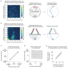
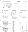
Figure 3. Habitual, egocentric movements do not explain the spatial memory for escape

a, Examples of homing runs – continuous turn-and-run movements toward the shelter – extracted from all movement data (Supplementary Video 9; Methods). Turn angles are defined as the difference in heading direction between the homing initiation point and the point where the mouse has travelled 15 cm. Turn angles are positive for rightward turns and negative for leftward turns. b, Predicting the escape targets of mice in the CORE-ZB on the basis of their previous turning movements. Left: diagram illustrating the method for predicting the escape target based on the turn angles from previous homing runs. Right: the y-axis measures the amount of variance in escape targets across trials that can be explained by mice repeating turn angles from previous homing runs. The positive control is a platform with narrow corridors, in which movements are stereotyped (see Extended Data Fig. 5; N=30 escapes, 10 mice). The test condition is the CORE-ZB. The negative control is predicting a random angle, and then extrapolating that angle to predict escape targets in the CORE-ZB (avg R² from doing this 1000 times). c, An experiment similar to the CORE-ZB, but with an additional barrier present during exploration. N=20 escapes, 10 mice. Bottom: distribution of turn angles from homing movements and from escapes. Both sets of angles are extracted in the same way (Fig. 3a; Methods). Black shows the new CORE with two barriers, and blue shows the two original COREs (Fig. 2A). Chi-square test comparing the angle distributions, binned as shown in the figure; exploratory movements: P=0.001 (**); escape movements: P=0.6. d, An experiment like the CORE-ZB, but in which the shelter is moved following the exploration period. N=18 escapes, 10 mice. Analysis is the same as in panel c. Bottom: Black shows the new CORE with the moved shelter, and blue shows the two original COREs. Chi-square test; exploratory movements: P=0.5; escape movements: P=0.03 (*).

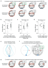
Figure 4. Mice memorize previously targeted subgoal locations

a, Correlation of different running movements with the escape target score, in the CORE-ZB. These include homing runs from the threat area to different parts of the obstacle, as well as runs from the shelter area to the obstacle edge. Movements toward the same edge targeted in the escape (here, the right edge) are considered separately from movements toward the opposite edge (here, the left). Boxes show the correlation coefficients and respective p-values; significant correlations have green outlines. b, Homing run history for two mice in the CORE-ZB, and subsequent escape trajectories. c, Escape targets plotted against the number of spontaneous edge-vector homing runs during exploration in the CORE-ZB. As shown in panel a, these only include movements toward the same edge targeted during the escape. d, Spatial efficiency of escapes on the first trial in the presence of an obstacle (same data as in Figure 1). As in previous panels, edge vectors only include movements to the edge targeted during the escape. Zero edge vectors: N=9 escapes, 9 mice; ≥1 edge vector: N=12 escapes, 12 mice. Two-sided permutation test: P=0.04 (*). e, Escape targets plotted against the number of spontaneous edge-vector homing runs during exploration, for acute obstacle removal on the first trial. f, Chronic obstacle removal experiment without a shelter present during the 20-min exploration period. All subsequent escapes are shown on the right. g, Chronic obstacle removal experiment with an extra barrier blocking the threat area during the 20-min exploration period. All subsequent escapes are shown on the right. h, Summary of escape targets in the two modified CORE-ZB experiments. One-sided permutation test on the proportion of edge-vector escapes, compared to the open-field condition (as in Fig. 2B). No shelter condition: N=24 escapes, 10 mice; Block threat side condition: N=25 escapes, 10 mice. White squares show the median, thick lines show the IQR, and thin lines show the range excluding outliers. Distributions are kernel density estimates.

Figure 5. Experience with an obstacle changes food-seeking but not exploratory trajectories

a, Food-approach paths in response to a 10-kHz tone associated with the availability of condensed milk at a reward port. An example trial is shown on top, and all paths are shown below. The red circle with ‘R’ represents the reward location, i.e. the metal spout with milk. The dotted line indicates the location of the obstacle during the initial 20-minute period. b, Summary data for food-seeking paths, computed the same way as escape targets. One-sided permutation test on the proportion of edge-vector paths: P=0.006 (**). Open field: N=32 reward runs, 6 mice; obstacle removed: N=34 reward runs, 6 mice. c, Paths across the platform during spontaneous exploration in the escape experiments. All paths go from the ends of the platform toward the center. Conditions with more sessions are randomly downsampled so that the same number of paths is displayed for each condition. d, The number of spontaneous center-directed and edge-directed movements during exploration. One-sided permutation test on the number of edge-directed movements; obstacle vs. open field: P=2x10^-5 (***); obstacle removed vs. open field: P=0.9. Obstacle: N=24 mice; obstacle removed (CORE with 0 and with 3 baseline trials): N=20 mice; open field: N=10 mice. White squares show the median, thick lines show the IQR, and thin lines show the range excluding outliers. Distributions are kernel density estimates.

References

1. Lima SL, Dill LM. Behavioral decisions made under the risk of predation: a review and prospectus. Can J Zool. 1990;68:619–640.
1. Drickamer Lee C, Stuart J. Peromyscus: Snow Tracking and Possible Cues Used for Navigation. American Midland Naturalist. 1984;111:202.
1. McMillan BR, Kaufman DW. Travel path characteristics for free-living white-footed mice (Peromyscus leucopus) Can J Zool. 1995;73:1474–1478.
1. Benhamou S. An analysis of movements of the wood mouse Apodemus sylvaticus in its home range. Behavioural Processes. 1991;22:235–250. - PubMed
1. Thompson SD. Spatial Utilization and Foraging Behavior of the Desert Woodrat, Neotoma lepida lepida. Journal of Mammalogy. 1982;63:570–581.
Publication types
LinkOut - more resources