Modeling the Effects of Future Hydroclimatic Conditions on Microbial Water Quality and Management Practices in Two Agricultural Watersheds

Abstract

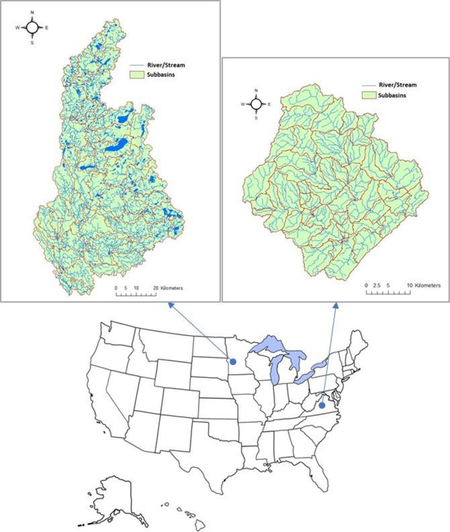
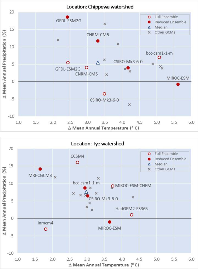
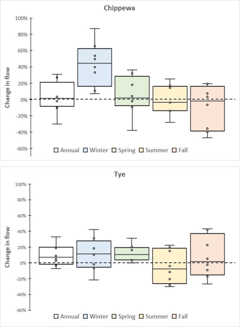
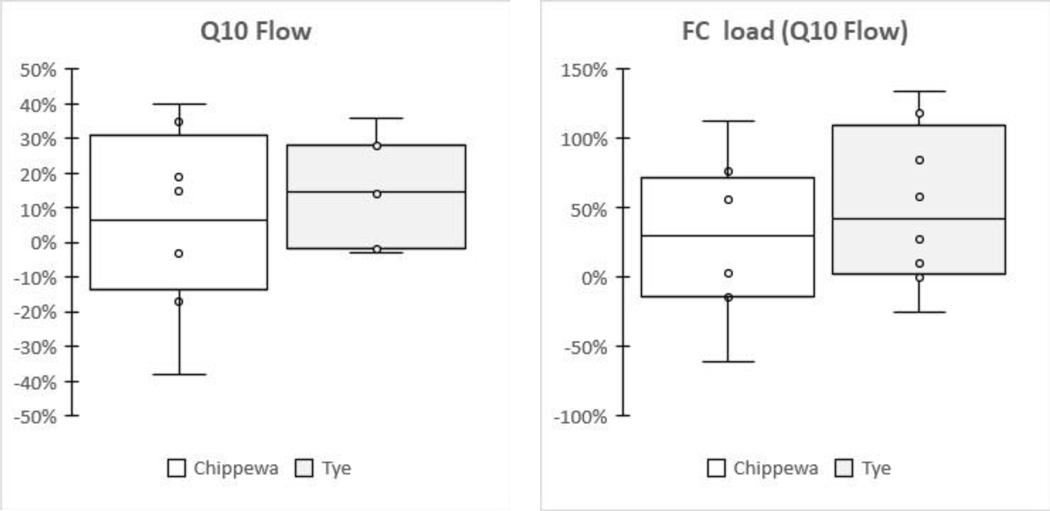
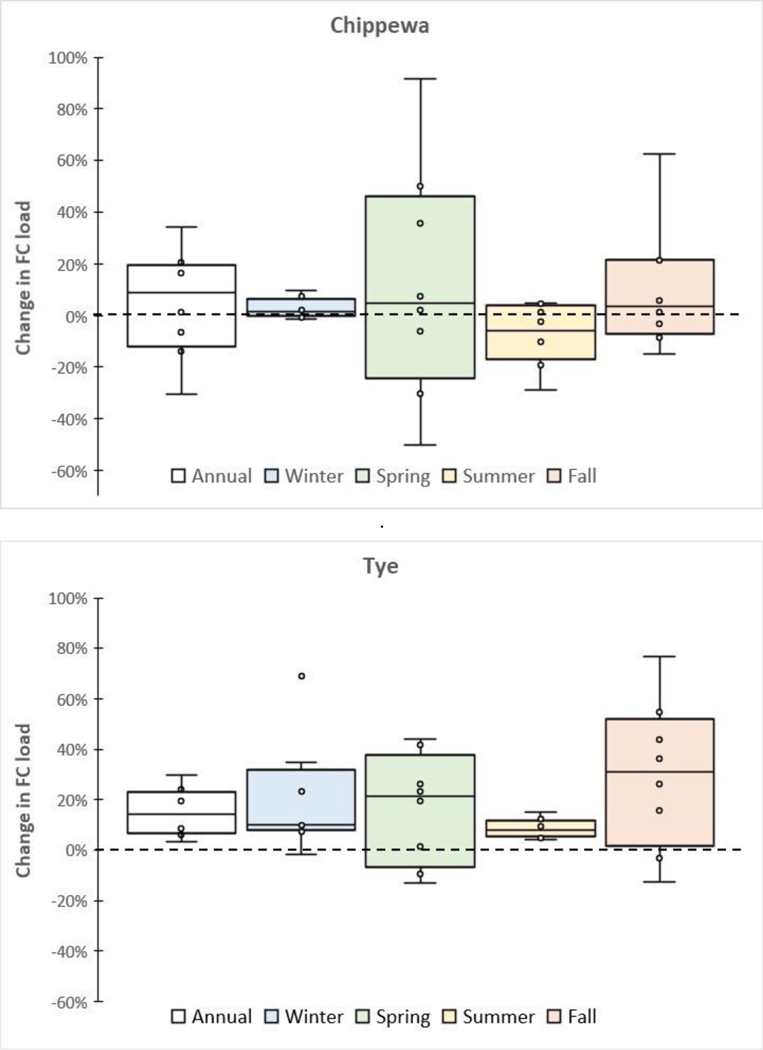
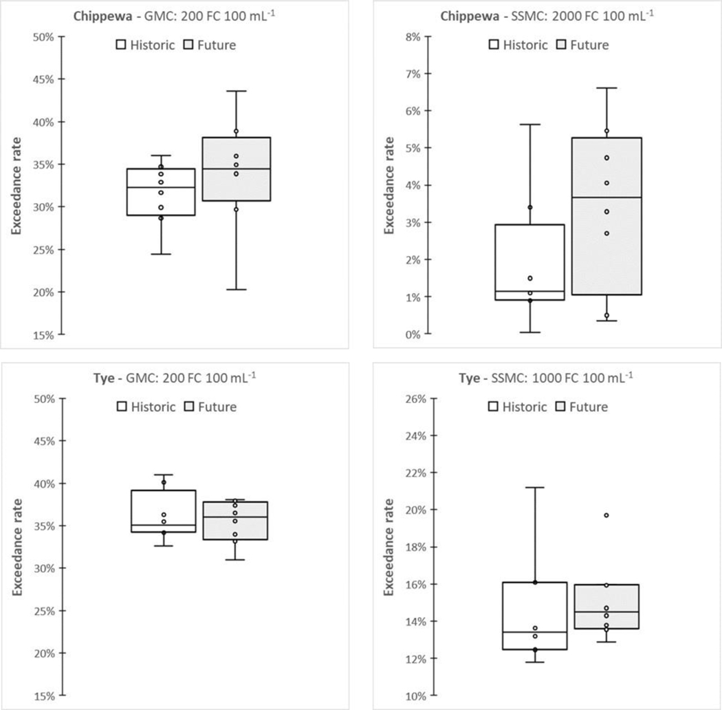
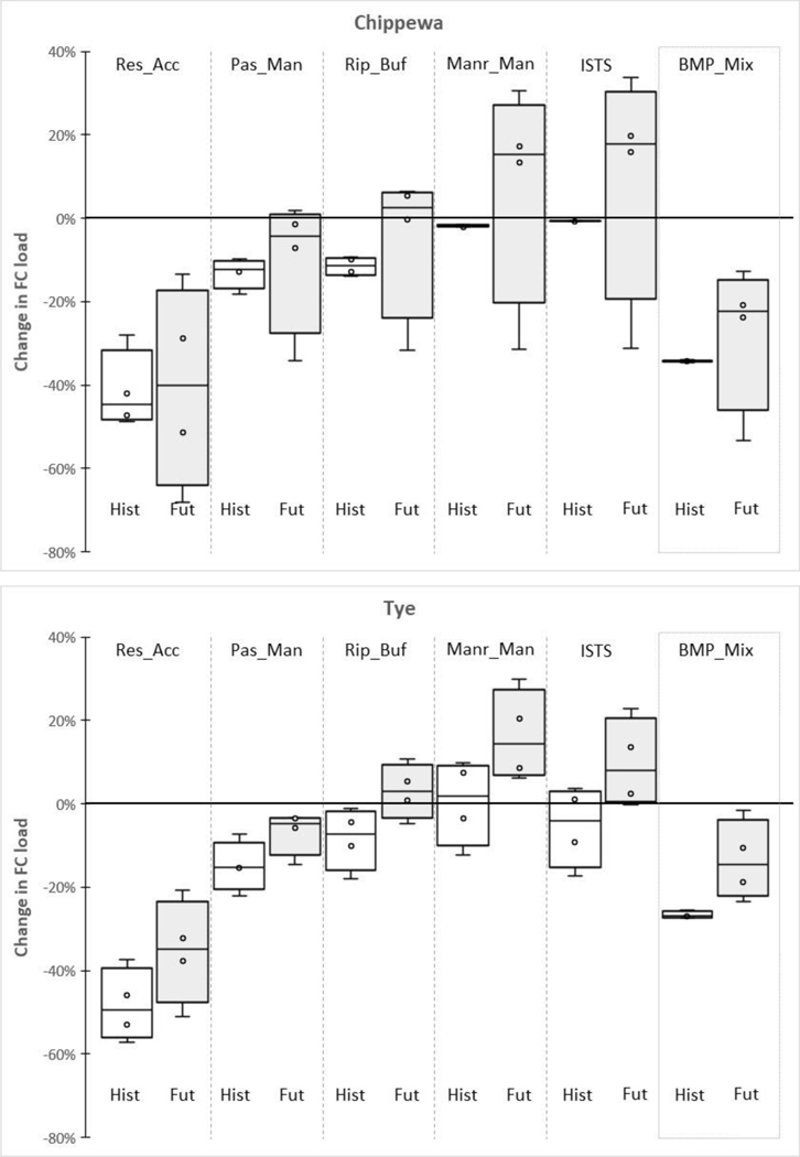
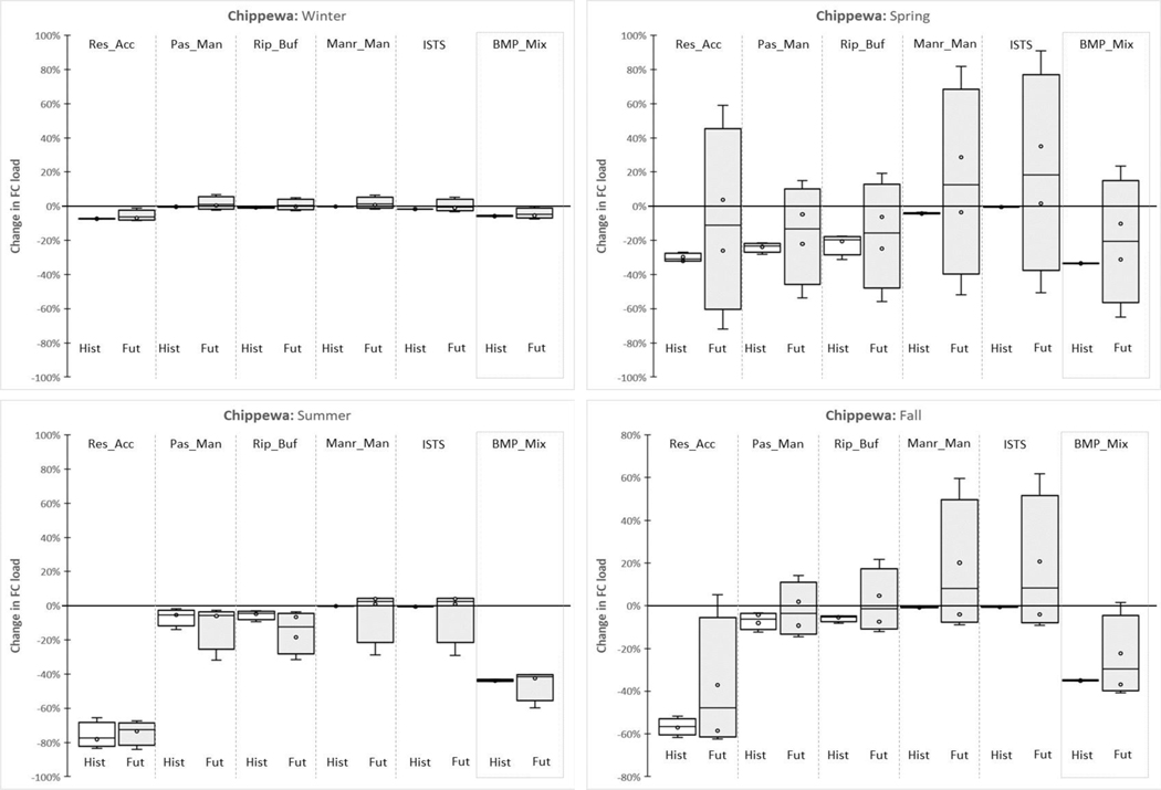
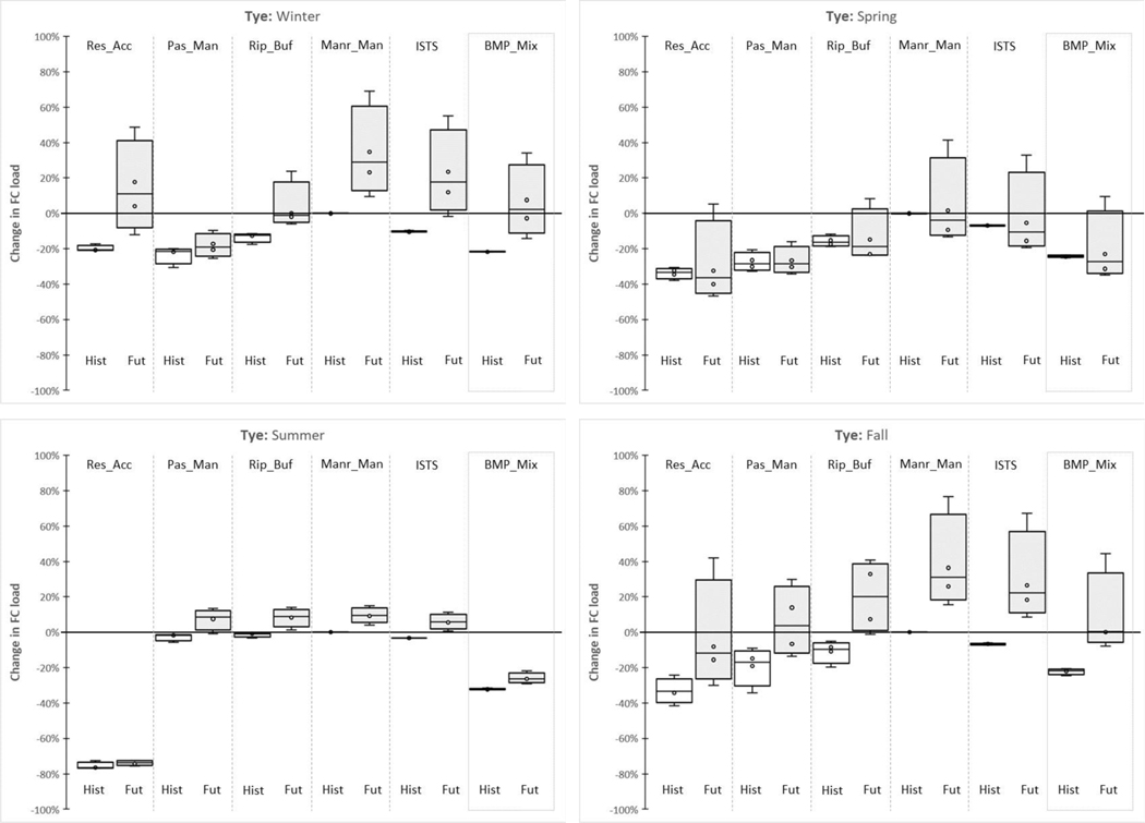
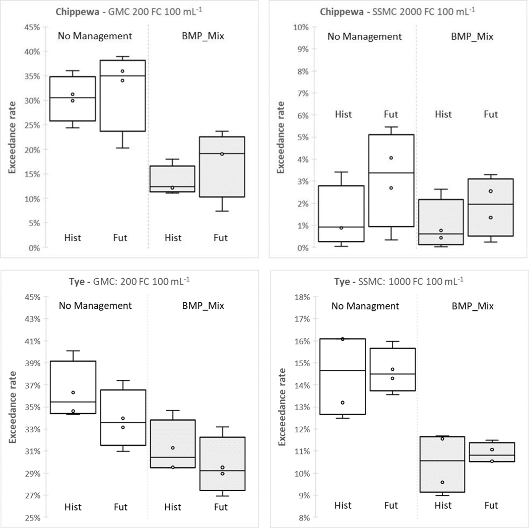
Anticipated future hydroclimatic changes are expected to alter the transport and survival of fecally-sourced waterborne pathogens, presenting an increased risk of recreational water quality impairments. Managing future risk requires an understanding of interactions between fecal sources, hydroclimatic conditions and best management practices (BMPs) at spatial scales relevant to decision makers. In this study we used the Hydrologic Simulation Program FORTRAN to quantify potential fecal coliform (FC - an indicator of the potential presence of pathogens) responses to a range of mid-century climate scenarios and assess different BMP scenarios (based on reduction factors) for reducing the risk of water quality impairment in two, small agricultural watersheds - the Chippewa watershed in Minnesota, and the Tye watershed in Virginia. In each watershed, simulations show a wide range of FC responses, driven largely by variability in projected future precipitation. Wetter future conditions, which drive more transport from non-point sources (e.g. manure application, livestock grazing), show increases in FC loads. Loads typically decrease under drier futures; however, higher mean FC concentrations and more recreational water quality criteria exceedances occur, likely caused by reduced flow during low-flow periods. Median changes across the ensemble generally show increases in FC load. BMPs that focus on key fecal sources (e.g., runoff from pasture, livestock defecation in streams) within a watershed can mitigate the effects of hydroclimatic change on FC loads. However, more extensive BMP implementation or improved BMP efficiency (i.e., higher FC reductions) may be needed to fully offset increases in FC load and meet water quality goals, such as total maximum daily loads and recreational water quality standards. Strategies for managing climate risk should be flexible and to the extent possible include resilient BMPs that function as designed under a range of future conditions.

Keywords: Climate; Management responses; Microbial water quality; Modeling; Watersheds.

Figure 1.

The Chippewa watershed, MN and the Tye watershed, VA.

Figure 2.

A summary of projected future mid-century air temperature and precipitation changes in the Chippewa watershed and Tye watershed for 8 GCM projections (represented by circles). The “Reduced Ensemble” is used for management scenario simulations. “Median” is calculated based on the “Full Ensemble”. Changes displayed are based on data from MACAv2-METADATA and further information (e.g., full GCM names) can be found at: https://climate.northwestknowledge.net/MACA/.

Figure 3.

Projected future changes in streamflow in the Chippewa and Tye watersheds. Percent change values are relative to the simulated 30-year baseline (1975–2005) for each model. Box and whisker plots show max and min (whiskers), 25^th, 50^th and 75^th percentiles (box) and individual values for each GCM (circles). Additional information about projected streamflow changes is provided in the online supporting information. Winter: Dec, Jan, Feb; Spring: Mar, Apr, May; Summer: Jun, Jul, Aug; Fall: Sep, Oct, Nov.

Figure 4.

Projected future changes in Q10 streamflow and FC load (under Q10 conditions) in the Chippewa and Tye watersheds. Percent change values are relative to the simulated 30-year baseline (1975–2005) for each model. Box and whisker plots show max and min (whiskers), 25^th, 50^th and 75^th percentiles (box) and individual values for each GCM (circles). Details about changes associated with individual GCMs are provided in the online supporting information.

Figure 5.

Projected future changes in average FC load in the Chippewa and Tye watersheds. Percent change values are relative to the simulated 30-year baseline (1975–2005) for each model. Box and whisker plots show max and min (whiskers), 25^th, 50^th and 75^th percentiles (box) and individual values for each GCM (circles). Details about changes associated with individual GCMs are provided in the online supporting information. Winter: Dec, Jan, Feb; Spring: Mar, Apr, May; Summer: Jun, Jul, Aug; Fall: Sep, Oct, Nov.

Figure 6.

Recreational water quality criteria exceedances rates for historic (baseline) and future conditions in the Chippewa and Tye watersheds. Values for historical are simulated baseline for each model, and not observed. GMC = Geometric mean concentration; SSMC = Single sample maximum concentration. Box and whisker plots show max and min (whiskers), 25^th, 50^th and 75^th percentiles (box) and individual values for each GCM (circles). Note: Chippewa exceedance rates are for the April to October period.

Figure 7.

Changes in annual fecal coliform load for 6 management scenarios relative to the historic baseline (1975–2005) in the Chippewa and Tye watersheds. Box and whisker plots show max and min (whiskers), 25^th, 50^th and 75^th percentiles (box) and individual values for each GCM (circles). Details about changes associated with specific GCMs are provided in the online supporting information. Values for historical are simulated 30-year baseline (1975–2005) for each model, and not observed.

Figure 8.

Changes in seasonal (meteorological) fecal coliform load for 6 management scenarios relative to the historic baseline (1975–2005) in the Chippewa watershed. Details about changes associated with specific GCMs are provided in the online supporting information. Box and whisker plots show max and min (whiskers), 25^th, 50^th and 75^th percentiles (box) and individual values for each GCM (circles). Values for historical are simulated 30-year baseline (1975–2005) for each model, and not observed. Winter: Dec, Jan, Feb; Spring: Mar, Apr, May; Summer: Jun, Jul, Aug; Fall: Sep, Oct, Nov.

Figure 9.

Seasonal changes in FC load for 6 management scenarios relative to the historic baseline (1975–2005) in the Tye watershed. Details about changes associated with specific GCMs are provided in the online supporting information. Box and whisker plots show max and min (whiskers), 25^th, 50^th and 75^th percentiles (box) and individual values for each GCM (circles). Values for historical are simulated 30-year baseline (1975–2005) for each model, and not observed. Winter: Dec, Jan, Feb; Spring: Mar, Apr, May; Summer: Jun, Jul, Aug; Fall: Sep, Oct, Nov.

Figure 10.

Recreational water quality criteria exceedances rates for the 30-year historic baseline and future periods, and a mixed BMP scenario (historic and future). GMC = Geometric mean concentration; SSMC = Single sample maximum concentration. Values for historical are simulated 30-year baseline (1975–2005) for each model, and not observed. Box and whisker plots show max and min (whiskers), 25^th, 50^th and 75^th percentiles (box) and individual values for each GCM (circles). Note: Chippewa exceedance rates are for the April to October period.

References

-
- Abatzoglou JT, & Brown TJ (2012). A comparison of statistical downscaling methods suited for wildfire applications. International Journal of Climatology, 32(5), 772–780. doi:10.1002/joc.2312 - DOI
- Agouridis CT, Workman SR, Warner RC, & Jennings GD (2005). LIVESTOCK GRAZING MANAGEMENT IMPACTS ON STREAM WATER QUALITY: A REVIEW1. JAWRA Journal of the American Water Resources Association, 41(3), 591–606. doi:10.1111/j.1752-1688.2005.tb03757.x - DOI
- Baffaut C. (2010). Bacteria Modeling with SWAT for Assessment and Remediation Studies: A Review. Transactions of the ASABE, v. 53(no. 5), pp. 1585–1594-2010 v.1553 no.1585. Retrieved from http://asae.frymulti.com/toc_journals.asp?volume=53&issue=5&conf=t&orgco...
- Benham BL, Baffaut C, Zeckoski RW, Mankin KR, Pachepsky YA, Sadeghi AM, … Habersack MJ (2006). MODELING BACTERIA FATE AND TRANSPORT IN WATERSHEDS TO SUPPORT TMDLS. Transactions of the ASABE, 49(4), 987–1002. doi:10.13031/2013.21739 - DOI
Grants and funding
LinkOut - more resources
Full Text Sources