High-Throughput Feeding Bioassay for Lepidoptera Larvae

Abstract

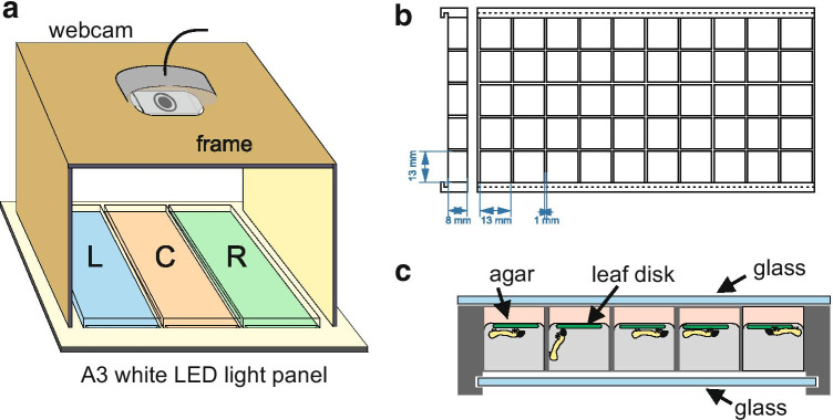
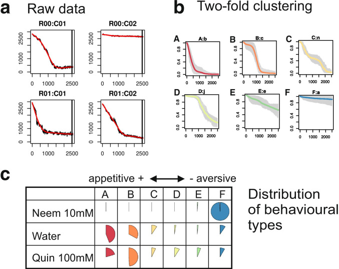
Finding plant cultivars that are resistant or tolerant against lepidopteran pests, takes time, effort and is costly. We present here a high throughput leaf-disk consumption assay system, to screen plants for resistance or chemicals for their deterrence. A webcam capturing images at regular intervals can follow the feeding activities of 150 larvae placed into individual cages. We developed a computer program running under an open source image analysis program to analyze and measure the surface of each leaf disk over time. We further developed new statistical procedures to analyze the time course of the feeding activities of the larvae and to compare them between treatments. As a test case, we compared how European corn borer larvae respond to a commercial antifeedant containing azadirachtin, and to quinine, which is a bitter alkaloid for many organisms. As expected, increasing doses of azadirachtin reduced and delayed feeding. However, quinine was poorly effective at the range of concentrations tested (10^-5 M to 10^-2 M). The model cage, the camera holder, the plugins, and the R scripts are freely available, and can be modified according to the users' needs.

Keywords: Digital image analysis; Feeding preferences; High-throughput device; Plant–insect warfare.

Fig. 1

Diagram of the feeding bioassay. a. One feeding bioassay setup corresponds to one batch, includes three 50-cages plates numbered L (left), C (center), R (right), and a webcam connected to a computer through a USB port. A white LED lightning board illuminates the plates from underneath b. Diagram of a 3D printed plate with 50 cages (13 × 13 × 8 mm) viewed from above and from the side. Longitudinal grooves are present on one face to slide in a glass plate. The other side’s glass plate is placed close to the cages frame and maintained to it with rubber bands. c. Profile view of one plate covered with two transparent glasses and showing larvae feeding on leaf disks. A 3–5 mm layer of 1% agar is first deposited on the bottom of the cage, and 1 cm diameter leaf disks freshly punched from a plant are deposited on the agar. Then, the larvae are introduced into the individual cages row by row and enclosed in their cages by sliding a second glass plate over the filled cages. The system is then placed upside down on the light panel so that the camera is able to monitor the disks through the layer of agar with little interference from the larvae crawling inside the cages

Fig. 2

Image analysis workflow. a. The first step of the analysis is to define an array of regions of interest (ROIs) defining the limit of each cage. This is done interactively under ICY, using a custom plugin RoitoRoiArray. On this picture, only one plate is displayed with the ROIs in place (yellow). b. The second step is to choose a filter procedure and a threshold adapted to detect the leaf disks, based on the intensity of the filtered image (obtained by combining the 3 color planes) or based upon a color space defined by points sampled by the user over the image. The corresponding area is overlayed in red over the original image. On this figure, we have selected and zoomed over 4 cages at the beginning and at the end of an experiment. The whole stack of images is then analyzed to measure the number of corresponding pixels in each ROI. The filtering and measuring (and data export) are done interactively under ICY, using a custom plugin AreaTrack c. Evolution of the surface of the 4 disks represented in Fig. 2b

Fig. 3

Data analysis workflow under R. a. Raw data processing. The surfaces measured in pixels are exported as a table (column = ROI, row = time) and displayed as an array curves using the same disposition as the plates. Here, 4 of such curves are displayed corresponding to the raw experimental data of Fig. 2c, with time in abscissa, and the number of pixels as ordinates. Each figure displays the raw data (black curve) and a filtered curve over it (in red). These curves are printed to pdf files to let the user check visually the quality of the results. The tables are then transposed (ROI = row, time = column) and further analyzed with R procedures. b. Two-fold clustering. First, SOTA classification results into 14 clusters. Each cluster is represented by a vignette showing the median consumption curve (color line) and the variations around the median at each time point (grey area). Second, SOTA clusters are grouped into six types using the median value of characteristic times t20, t50, t80 and total consumption representing the clusters. At the end, the consumption curve of each cage is attributed a behavioural type, between A and F. c. Results: distribution of behavioural types for each treatment. As an example, we show here the distribution of behavioural types in three treatments: NeemAzal 10 mM, Water (control), and Quinine 100 mM. The frequency of types (A to F) in each category (column: type, row: stimulus) is represented as a pie chart. Each row sums to 1

Fig. 4

Distribution of behavioural types for the different treatments. For each treatment (column), the estimated probability of each behavioural type is represented as a pie. Each column sums to one. a. Neemazal treatments. Neemazal concentrations are reported as legend to each column. « None» corresponds to the control with water. b. Quinine treatments. Quinine concentrations are indicated in the column names. « None» corresponds to the control with water. The colour gradient corresponds to appetitive (red) to aversive (blue)

References

1. Adesanya AW, Morales MA, Walsh DB, Lavine LC, Lavine MD, Zhu F. Mechanisms of resistance to three mite growth inhibitors of Tetranychus urticae in hops. Bull Entomol Res. 2018;108:23–34. doi: 10.1017/s0007485317000414. - DOI - PubMed
1. Aguirre-Liguori JA, et al. Divergence with gene flow is driven by local adaptation to temperature and soil phosphorus concentration in teosinte subspecies (Zea mays parviglumis and Zea mays mexicana) Mol Ecol. 2019;28:2814–2830. doi: 10.1111/mec.15098. - DOI - PubMed
1. Akaike H (1998) Information theory and an extension of the maximum likelihood principle. In: Parzen E, Tanabe K, Kitagawa G, Parzen E, Tanabe K, Kitagawa G (eds) Selected Papers of Hirotugu Akaike. New York, NY, pp 199–213. 10.1007/978-1-4612-1694-0_15
1. Alchanatis V, Navon A, Glazer I, Levski S. An image analysis system for measuring insect feeding effects caused by biopesticides. J Agr Eng Res. 2000;77:289–296. doi: 10.1006/jaer.2000.0610. - DOI
1. Arnason JT, et al. Antifeedant and insecticidal properties of azadirachtin to the European corn borer, Ostrinia nubilalis. Entomol Exp Appl. 1985;38:29–34. doi: 10.1111/j.1570-7458.1985.tb03494.x. - DOI
LinkOut - more resources