Intravital fluorescence microscopy with negative contrast

Abstract

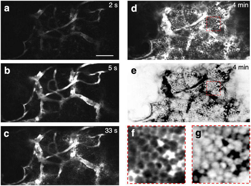
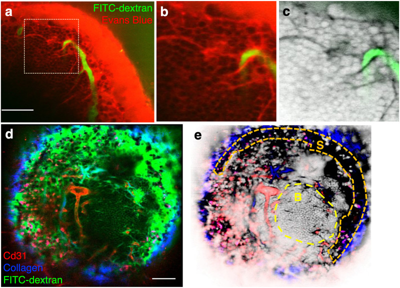
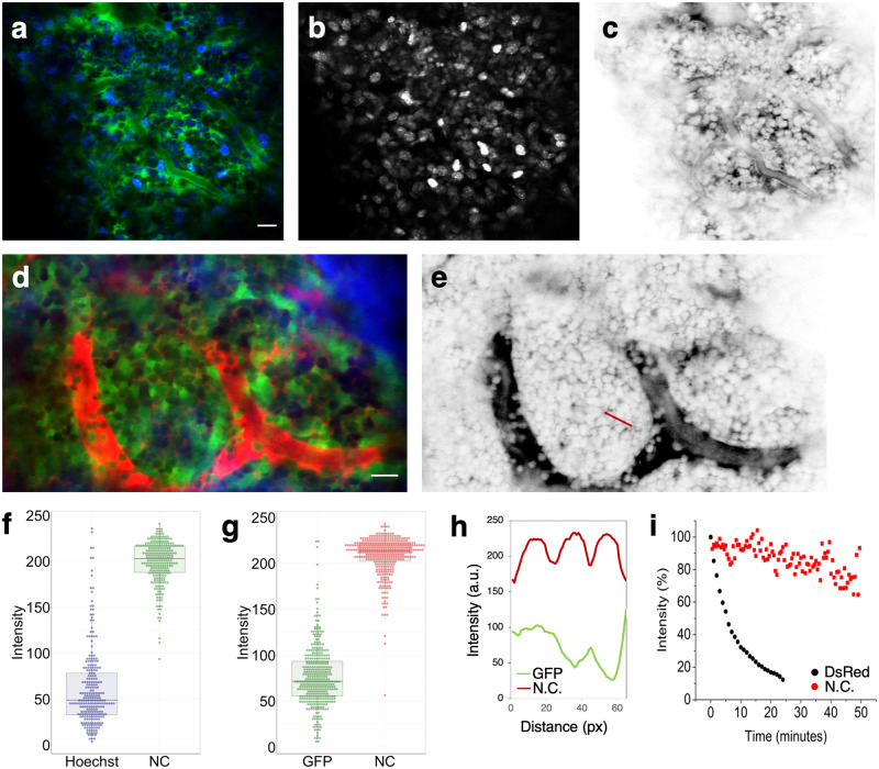
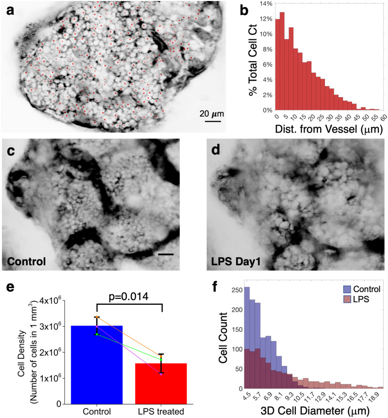
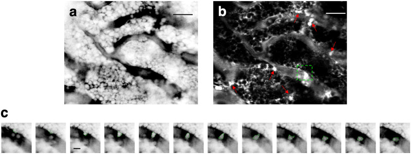
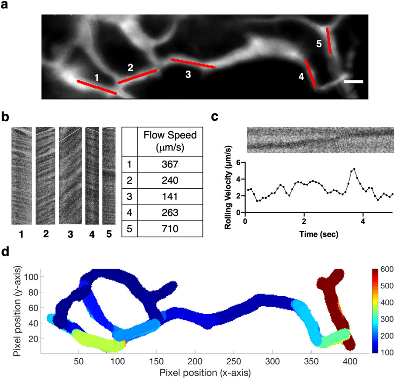
Advances in intravital microscopy (IVM) have enabled the studies of cellular organization and dynamics in the native microenvironment of intact organisms with minimal perturbation. The abilities to track specific cell populations and monitor their interactions have opened up new horizons for visualizing cell biology in vivo, yet the success of standard fluorescence cell labeling approaches for IVM comes with a "dark side" in that unlabeled cells are invisible, leaving labeled cells or structures to appear isolated in space, devoid of their surroundings and lacking proper biological context. Here we describe a novel method for "filling in the void" by harnessing the ubiquity of extracellular (interstitial) fluid and its ease of fluorescence labelling by commonly used vascular and lymphatic tracers. We show that during routine labeling of the vasculature and lymphatics for IVM, commonly used fluorescent tracers readily perfuse the interstitial spaces of the bone marrow (BM) and the lymph node (LN), outlining the unlabeled cells and forming negative contrast images that complement standard (positive) cell labeling approaches. The method is simple yet powerful, offering a comprehensive view of the cellular landscape such as cell density and spatial distribution, as well as dynamic processes such as cell motility and transmigration across the vascular endothelium. The extracellular localization of the dye and the interstitial flow provide favorable conditions for prolonged Intravital time lapse imaging with minimal toxicity and photobleaching.

Fig 1. Two-photon negative contrast imaging of a mouse BM cavity, at different time points after the injection of a vascular dye.

a–d, Images taken at 2 s, 5 s, 33 s and 4 min after tail-vein injection of 70 kDa Texas Red-dextran, respectively. Vascular signal was detected 2–5 s after injection. Leakage of the dye into the extravascular space could be seen by 33 s. By 4 min, the dye occupied the interstitial space between cells, which remained as dark objects in the image. e, The LUT of (d) was digitally inverted such that cells appeared as bright objects above the dark interstitial background. f-g, The dotted areas in (d,e) were magnified to show how individual cells appear in negative contrast imaging. Scale bar = 50 μm. Representative example from N = 3 mice.

Fig 2. Two-photon negative contrast imaging of the popliteal lymph node.

a, Interstitium labeling via lymphatic drainage. Evans blue (red) was delivered at a distant site (footpad) and into the popliteal LN via the lymphatic system. FITC-dextran (green) was injected intravenously to visualize the blood vessels. b, Zoomed-in view of the dotted region in (a), showing dark individual cells above the fluorescent interstitial background. Small vessel-like structures are lymphatic conduits that branch from the subcapsular sinus. c, Same as (b), after LUT inversion. N = 1 mouse. d, Popliteal lymph node imaged by a combination of negative contrast imaging of the follicular B cells, positive contrast imaging of the lymphatic vessels and vasculature, and second harmonic generation imaging of the LN capsule. FITC-dextran (green) was injected into footpad for lymphatic vessels and interstitium labeling. Anti CD31-Alexa 594 (red) was injected intravenously for vascular labeling. The SHG signal from the capsule is shown in blue. Punctate labeling in red is due to non-specific antibody uptake by macrophages. e, Same as (d), but with the green channel‘s LUT inverted and displayed in grayscale. The dotted area designated “S” indicates the position of the lymphatic sinus and the area designated “B”, the B cell follicle. Negative contrast imaging renders the cells in the follicle readily visible. N = 1 mouse. Scale bar for all images = 50 μm.

Fig 3. Comparison of negative contrast imaging with standard “universal” fluorescence labeling methods.

a, Colocalized image of BM cells, labeled with Hoechst 33342 (blue) and interstitial space, labeled with TRITC-dextran (green). b, The Hoechst channel shown in gray scale. c, The TRITC channel in gray scale after LUT inversion. N = 2 mice. d, Colocalized image of BM cells expressing actin-GFP (green) and interstitial space labeled by rhodamine B-dextran (red). Bone second-harmonic generation signal is shown in blue. e, The rhodamine B channel in gray scale after LUT inversion. N = 1 mouse with 6 different z-stack locations. f, Boxplots of cell intensities in (a). 226 cells were included. g, Boxplots of cell intensities in (d). 369 cells were included. h, GFP (green) and negative contrast (red) intensity profiles along the red line marked in (e), which spans the width of 3 cells. The negative contrast profile is more consistent than the GFP profile from cell to cell, and the cell boundaries are well-defined. i, Photobleaching kinetics of actin-DsRed labeled cells (black) and FITC-dextran labeled interstitium (red). Signal was acquired from BM in vivo, and the excitation laser was continuously scanned over the field of imaging during signal acquisition. N = 2 mice. Scale bar for all images = 20 μm.

Fig 4. Quantitative analysis of cell locations, density and sizes using negative contrast imaging.

a, Negative contrast image of a BM cavity, 10 μm below the endosteum. Centroid of each cell is marked as a red dot. The centroids of some cells are at other z-depths (full 3D stack is shown in S3 Movie). b, Histogram of the Euclidean distance between the cell centroids to their nearest blood vessel wall. ~90% of the cells are within 30 μm to the nearest blood vessel. N = 4 mice. c-d, Representative negative contrast image of the same BM cavity before and one day after LPS treatment. N = 3 mice (total of 18 z-stack locations) e, Comparison of cell density measured before and one day after LPS treatment (N = 2 mice, total of 3 z-stack locations). Significant decrease in cell density was observed after LPS treatment. Statistical analysis was performed by using paired sample t test (p value = 0.014). f, Histogram of cell sizes in a BM cavity before (blue) and one day after (red) LPS treatment. Scale bar for all images = 20 μm.

Fig 5. Visualizing BM cell dynamics by negative contrast imaging.

a, A single snapshot from a time-lapse negative contrast imaging sequence of a mouse BM (the sequence is shown in S6 Movie). b, A standard deviation image created from the time lapse sequence. Bright regions with high standard deviation values are indicated by red arrows. These areas correspond to the regions of high cell motility. The dotted rectangle indicates the location of a transendothelial migration event. Scale bar = 30 μm. c, Time lapse negative contrast images of a cell transmigrating across the endothelial wall. The boundary of the cell is indicated by a green dotted line. Consecutive images were taken 30 seconds apart. Scale bar = 5 μm. Representative of N = 5 mice.

Fig 6. Automated blood flow profiling with negative contrast time series.

a, The vascular network used for automated blood flow profiling, as an averaged image of the 120 fps, 2 s long negative contrast time series (S9 Movie). Scale bar = 20 μm. b, Digital line scan image for each red-marked vessel segment in (a). Conceptually, each image is a vertical montage of the segment imaged at consecutive time points; a stationary cell would display as a vertical dark stripe. The slope of the stripes was estimated by Radon transform and overlaid on the images in white. Blood flow speeds were calculated from the slope value. c, Change in rolling lymphocyte velocity calculated over time. The raw digital line scan image shows the shadow of the rolling lymphocyte moving along the vessel (top). The velocity was calculated every 0.1 seconds at 30 fps. d, Flow profile of the 2D vascular network shown in (a), generated by automated vessel segment selection and local flow speed mapping. Speed scale is in μm/s. N = 5 mice.

References

1. Jain RK, Munn LL, Fukumura D. Dissecting tumour pathophysiology using intravital microscopy. Nat Rev Cancer. 2002;2: 266–276. doi: 10.1038/nrc778 - DOI - PubMed
1. Pittet MJ, Weissleder R. Intravital Imaging. Cell. 2011;147: 983–991. doi: 10.1016/j.cell.2011.11.004 - DOI - PMC - PubMed
1. Miller MJ, Hejazi AS, Wei SH, Cahalan MD, Parker I. T cell repertoire scanning is promoted by dynamic dendritic cell behavior and random T cell motility in the lymph node. Proc Natl Acad Sci. 2004;101: 998–1003. doi: 10.1073/pnas.0306407101 - DOI - PMC - PubMed
1. Qi H, Egen JG, Huang AYC, Germain RN. Extrafollicular activation of lymph node B cells by antigen-bearing dendritic cells. Science. 2006;312: 1672–1676. doi: 10.1126/science.1125703 - DOI - PubMed
1. Henrickson SE, Mempel TR, Mazo IB, Liu B, Artyomov MN, Zheng H, et al.. T cell sensing of antigen dose governs interactive behavior with dendritic cells and sets a threshold for T cell activation. Nat Immunol. 2008;9: 282–291. doi: 10.1038/ni1559 - DOI - PMC - PubMed
Publication types