Do Spectra Live in the Matrix? A Brief Tutorial on Applications of Factor Analysis to Resolving Spectral Datasets of Mixtures

Abstract

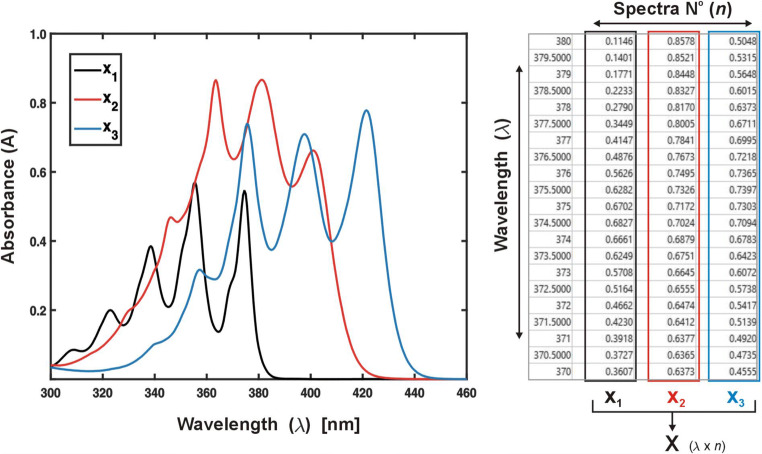
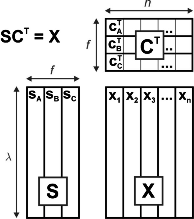
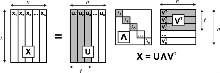
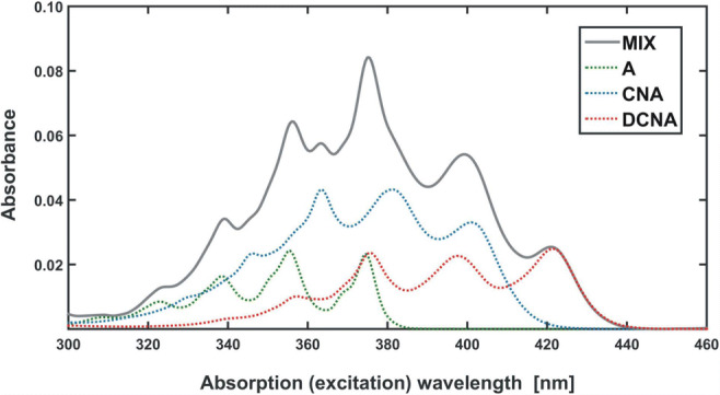
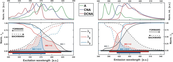
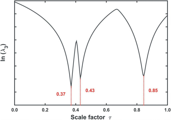
In spite of a rapid growth of data processing software, that has allowed for a huge advancement in many fields of chemistry, some research issues still remain problematic. A standard example of a troublesome challenge is the analysis of multi-component mixtures. The classical approach to such a problem consists of separating each component from a sample and performing individual measurements. The advent of computers, however, gave rise to a relatively new domain of data processing - chemometry - focused on decomposing signal recorded for the sample rather than the sample itself. Regrettably, still a very few chemometric methods are practically used in everyday laboratory routines. The Authors believe that a brief 'user-friendly' guide-like article on several 'flagship' algorithms of chemometrics may, at least partly, stimulate an increased interest in the use of these techniques among researchers specializing in many fields of chemistry. In the paper, five different techniques of factor analysis are used for the analysis of a three-component system of fluorophores. These algorithms, applied on the excitation-emission spectra, recorded for the 'unknown' mixture, allowed to unambiguously determine its composition without the need for physical separation of the components. An example of using chemometric methods for physical chemistry research is also provided. For each presented technique of the data analysis, a short description of its theoretical background followed by an example of its practical performance is given. In addition, the Reader is supplemented with a basic information on matrix algebra, detailed experimental 'recipes', reference specialist literature and ready-to-use MATLAB codes.

Keywords: Evolving factor analysis; Excitation-emission maps; Fluorescence quenching; Multivariate curve resolution; Rank annihilation factor analysis; Spectral data matrices of mixtures.

Fig. 1

Graphical (left) and matrix representation (right) of spectral data

Fig. 2

Scheme showing matrix formulation of Lambert-Beer law. The data matrix X, containing n spectra of a three-component mixture, is decomposed into the product of matrices S and C, respectively, consisting of individual spectral and concentration (intensity) profiles of all components

Fig. 3

Scheme showing the decomposition of data matrix X from Fig. 2 into the product of three matrices U, Λ and V^T with the SVD algorithm. Submatrices, to which these matrices may be reduced for the purpose of data reproduction are marked in grey

Fig. 4

Geometric interpretation of two- and three-component x_AB and x_ABC mixture spectra. All spectra (black dots) are represented by points located in the coordinate system defined by the ‘standard’ spectra of ‘pure’ components s_A, s_B and s_C. The coordinates (dashed lines) are identical to the scaling factors (concentrations) c_A, c_B and c_C

Fig. 5

Geometric interpretation of eigenvectors u, obtained by SVD of the data matrix X. An appropriate set of such orthogonal vectors allows to draw a coordinate system describing the experimental data points. This is particularly useful when the spectra s_A, s_B and s_C of pure’ components, and hence the ‘original’ axes of the system remain unknown (cf. Figure 4 - the ‘red’ remains the same, but have been rotated)

Fig. 6

Absorption spectrum of a model three-component mixture (MIX) with marked contributions of all components (A, CNA, DCNA)

Fig. 7

Fluorescence (continuous line), absorption (dotted line) and excitation (dashed line) spectra of the studied fluorophores normalised to a unit maximum

Fig. 8

Excitation-emission map recorded for a mixture of three fluorophores before (left) and after addition of potassium iodide as a quencher (right). In the emmision range of 300–380 nm, characteristic, protruding ‘sharp’ bands (originating from anthracene) can be observed

Fig. 9

Top: first four eigenvectors u obtained for dataset X_MIX (Fig. 8– left panel). The first three of them are characterized by a regular pattern, while the fourth one reflects a random, chaotic noise. At the bottom: the fluorescence spectra of the three mixture components (Fig. 7). A correlation can be seen between the abstract (top) and real (bottom) spectra (i.e. in extreme positions – see SI – App. A.3)

Fig. 10

Schematic diagram of the TFA procedure carried out for an ‘unknown’ sample and spectra of four ‘target’ substances: A, CNA, DCNA and DPhA (black lines). The first three of them are well reproduced by a combination of eigenvectors (red lines), which seems to confirm their presence in a mixture. For the spectrum of DPhA, this regularity does not exist, which indicates that it was not a component of the sample

Fig. 11

Excitation-emission map of CNA calibration sample before (A) and after (B) reproduction. On the difference map (C) a ‘rugged’ structure, representing instrumental noise, and Rayleigh scattering band residuals (marked with red lines and arrows) are observed. For comparison, a miniature of EEM of the pure solvent (methanol) is shown (D)

Fig. 12

Graphical visualisation of the iterative RAFA algorithm. The singular values λ obtained for the difference matrices D_MIX (12) are plotted against a set of the corresponding scaling parameters τ used for their construction. The optimal value τ₀ corresponds to a minimum value of the ‘last’ significant singular value (third). Just for comparison, the evolution of the second one is also shown. The applied logarithmic scale allows for easier observation of the extremes

Fig. 13

Schematic diagram of EFA. ‘Scanning’, that is stepwise augmentation of the analysed submatrix M may take place in two directions – forward or backward (from the shortest to longest wavelength or vice versa), and in two modes varying either the excitation or emission wavelength

Fig. 14

Curves normalized by their maximum values, showing the evolution of significant singular values of X_MIX as a function of the adopted range of the excitation (left) and emission wavelengths (right). Single component area is marked in grey (MIX 1), two component in red (MIX 1 + 2) and three component in blue (MIX 1 + 2 + 3). For comparison, at the top of the plots the spectra of individual mixture components are presented

Fig. 15

Excitation-emission map of the model mixture from Fig. 8 after determining the amount of significant factors by EFA method (Fig. 14). Spectra (black lines) coming from the marked in grey selective regions (MIX 1) are plotted on the side walls. Two-component regions are indicated in red (MIX 1 + 2) and three-component in blue (MIX 1 + 2 + 3)

Fig. 16

Graphical visualization of the iterative RAFA algorithm for a three-component system (A, CNA, and DCNA). The plot shows three minima of the third singular value. However, a direct correspondence with particular components is not established

Fig. 17

The fluorescence excitation (left) and emission spectra (right) obtained by GRAM technique (continuous lines) applied on the excitation-emission maps of the model mixture (Fig. 8). For the sake of comparison, the spectra measured individually for A, CNA and DCNA (dotted lines, Fig. 7) are also presented

Fig. 18

Stern-Volmer plots describing the fluorescence quenching process occurring in the analyzed mixture (Table 2). The data points were obtained by GRAM, RAFA ‘cascade’ and selective signal analysis. For comparison, the results of measurements conducted individually for ‘pure’ substances are also shown

Fig. 19

Example of ‘cascade’ RAFA procedure allowing to extract ‘pure’ spectra of all components by comparing three different datasets. In step one (upper panel), DCNA signal (recorded selectively) is annihilated (minimum of λ₂) from a two-component spectral dataset. Thus, individual spectra of CNA are obtained. In step two, DCNA and CNA contributions are subtracted from ternary spectra. As a result, ‘pure’ spectra of A are recovered. The subtraction can be performed either sequentially or simultaneously. In the first case, a three-component spectral dataset is deprived of DCNA contribution - λ₃ - and the resulting two-component spectral data matrix - of remaining CNA variance - λ₂’. In the second case, the contributions of both DCNA and CNA to a ternary mixture spectral dataset are estimated directly - 2 x λ₃)

References

1. Zinatloo-Ajabshir S, Heidari-Asil SA, Salavati-Niasari M. Simple and eco-friendly synthesis of recoverable zinc cobalt oxide-based ceramic nanostructure as high-performance photocatalyst for enhanced photocatalytic removal of organic contamination under solar light. Sep Purif Technol. 2021;267:118667. doi: 10.1016/j.seppur.2021.118667. - DOI
1. Rubio-Clemente A, Chica E, Peñuela GA. Rapid determination of anthracene and benzo (a) pyrene by high-performance liquid chromatography with fluorescence detection. Anal Lett. 2017;50:1229–1247. doi: 10.1080/00032719.2016.1225304. - DOI
1. Nie S, Dadoo R, Zare RN. Ultrasensitive fluorescence detection of polycyclic aromatic hydrocarbons in capillary electrophoresis. Anal Chem. 1993;65:3571–3575. doi: 10.1021/ac00072a007. - DOI
1. Malinowski ER, Howery DG. Factor analysis in chemistry. New York: Wiley; 1980.
1. Maeder M, Neuhold YM. Practical data analysis in chemistry. Amsterdam: Elsevier; 2007.
LinkOut - more resources