Dynamic mode decomposition in adaptive mesh refinement and coarsening simulations

Abstract

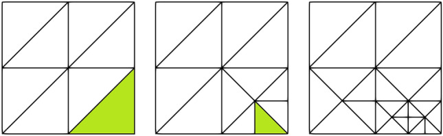
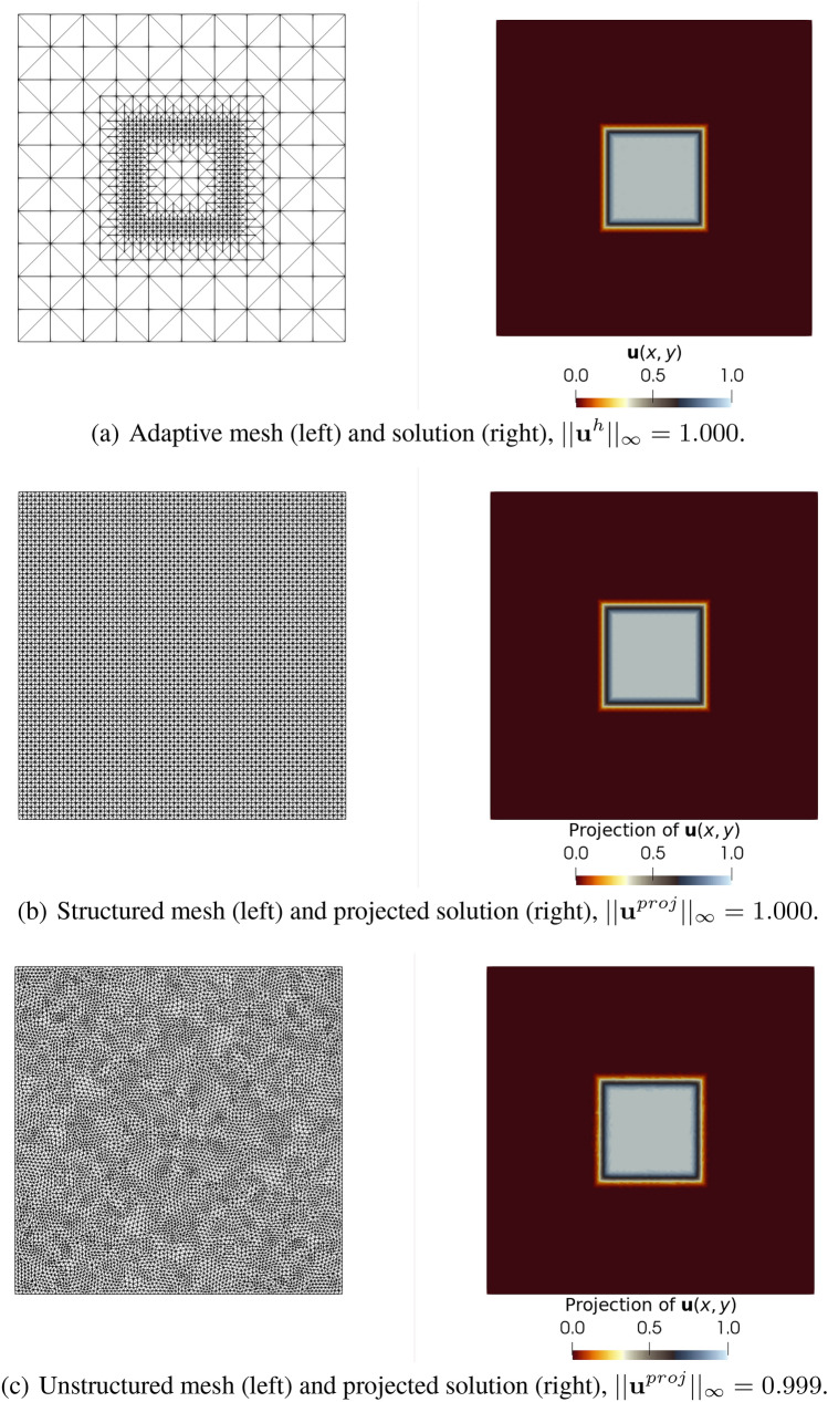
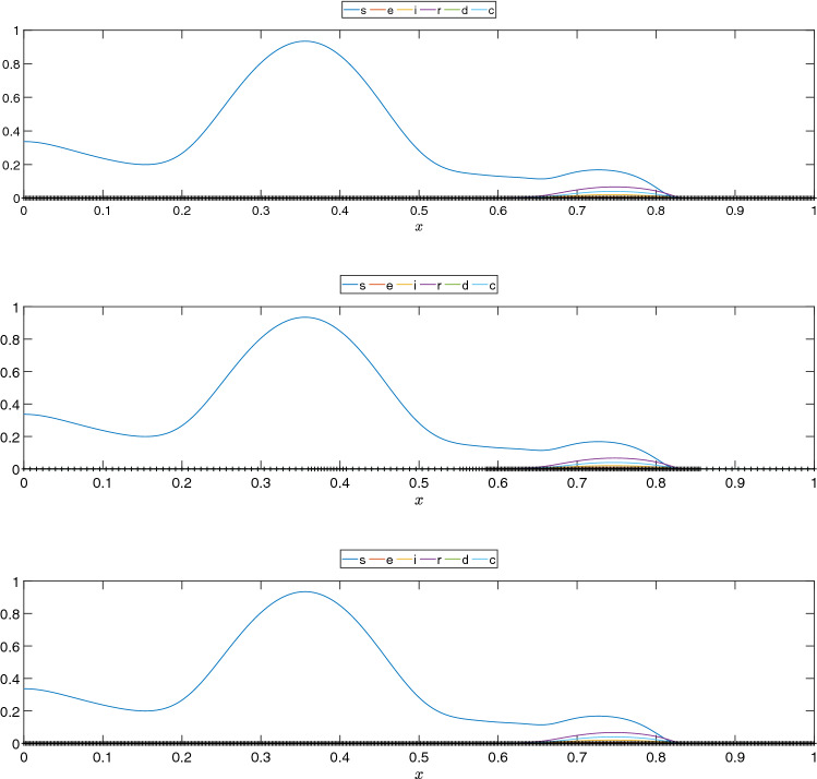
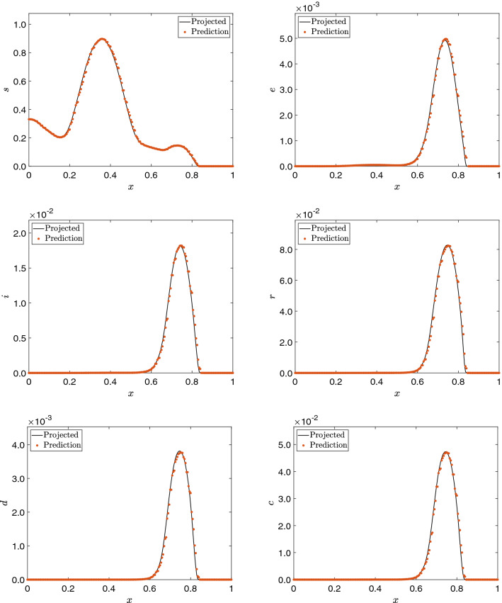
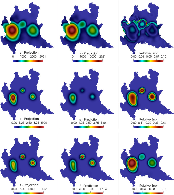
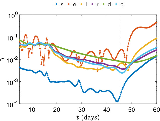
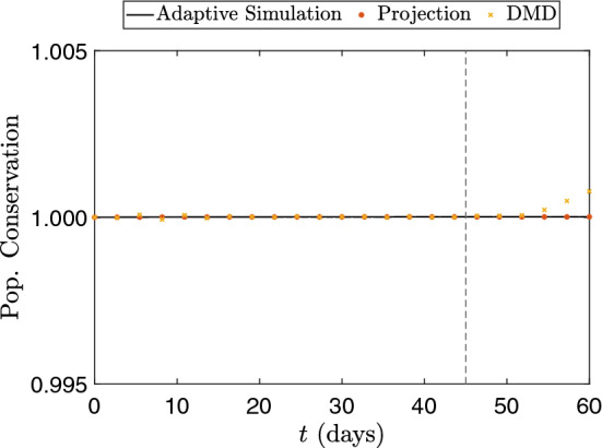
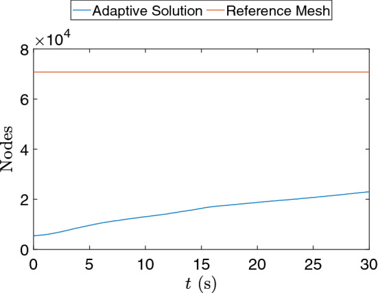
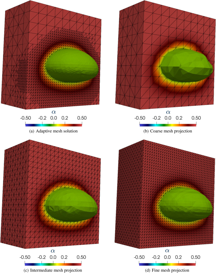
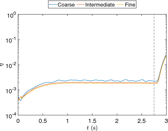
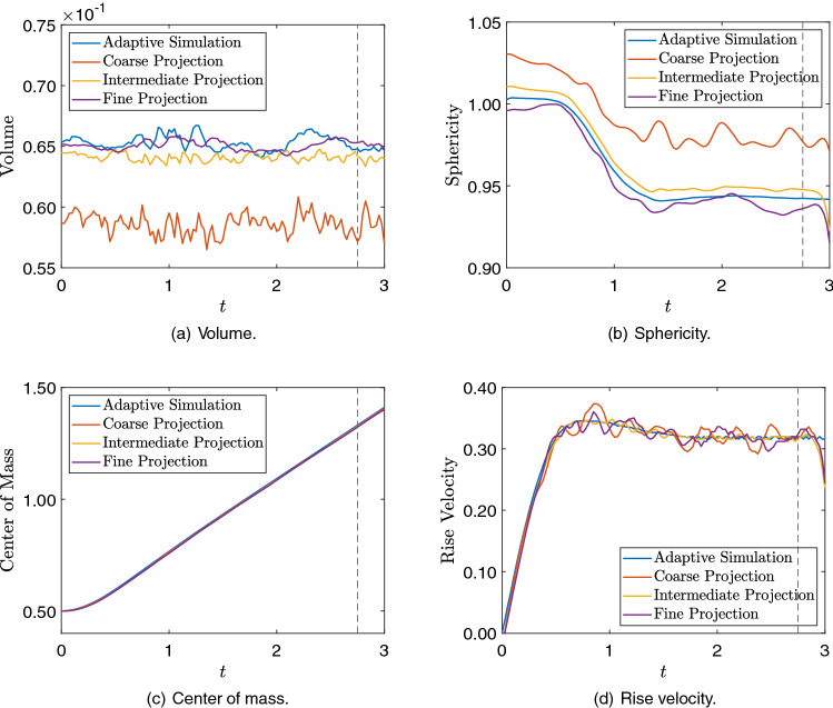
Dynamic mode decomposition (DMD) is a powerful data-driven method used to extract spatio-temporal coherent structures that dictate a given dynamical system. The method consists of stacking collected temporal snapshots into a matrix and mapping the nonlinear dynamics using a linear operator. The classical procedure considers that snapshots possess the same dimensionality for all the observable data. However, this often does not occur in numerical simulations with adaptive mesh refinement/coarsening schemes (AMR/C). This paper proposes a strategy to enable DMD to extract features from observations with different mesh topologies and dimensions, such as those found in AMR/C simulations. For this purpose, the adaptive snapshots are projected onto the same reference function space, enabling the use of snapshot-based methods such as DMD. The present strategy is applied to challenging AMR/C simulations: a continuous diffusion-reaction epidemiological model for COVID-19, a density-driven gravity current simulation, and a bubble rising problem. We also evaluate the DMD efficiency to reconstruct the dynamics and some relevant quantities of interest. In particular, for the SEIRD model and the bubble rising problem, we evaluate DMD's ability to extrapolate in time (short-time future estimates).

Keywords: Adaptive mesh refinement and coarsening; Dimensionality reduction; Dynamic mode decomposition; Mesh projection.

Fig. 1

Illustration of a mesh refinement procedure. A local a posteriori error estimator or indicator flags an element for refinement (in green) using the solution computed in the mesh on the left. The mesh is refined (or coarsened) according to the flagged elements, and the process can be restarted until a given criterion is met (error level, element size, maximum number of elements, etc.). Note that the initial and the final mesh differ in the number of degrees of freedom and topology

Fig. 2

Comparison of different ${\mathcal{L}}^2$-projection examples on structured and unstructured meshes

Fig. 3

Initial conditions for the 1D model

Fig. 4

Solution at $t=30$ days for the fixed mesh solution, AMR solution and the respective projection onto a reference mesh for the 1D SEIRD example. The reference mesh was built with characteristic length similar to the smaller elements in the adaptive mesh

Fig. 5

Solution at $t=44$ days for the AMR simulation solution and the 14 days projection using DMD for the 1D SEIRD example

Fig. 6

Number of mesh nodes in time for the adaptive solution and the proposed reference mesh for the 2D SEIRD example

Fig. 7

Initial conditions for the SEIRD model in the Lombardy case

Fig. 8

Solution for the susceptible compartment at $t=46$ days obtained using an adaptive mesh and its respective projection onto a fixed reference mesh

Fig. 9

Comparison between computed and predicted solutions at $t=60$ days for the susceptible, exposed, and infected compartments

Fig. 10

Comparison between computed and predicted solutions at $t=60$ days for the recovered, deceased, and cumulative infected compartments

Fig. 11

Relative error for all compartments between numerical simulation snapshots and DMD reconstruction and prediction. The dashed line represents the beginning of the DMD prediction stage

Fig. 12

Population conservation for both adaptive and projected results

Fig. 13

Scheme illustrating the initial conditions for the density-driven gravity flow example

Fig. 14

Results and mesh for the first 8 m of the domain at $t=10$s

Fig. 15

Number of mesh nodes in time for the adaptive solution and the proposed reference mesh for the density-driven gravity current example

Fig. 16

Relative error for the reconstruction considering different values of the rank r

Fig. 17

Front position and mass conservation for the fixed mesh and adaptive mesh simulations and reconstructions with the target mesh

Fig. 18

Initial configuration and boundary conditions for the bubble rising problem

Fig. 19

Level-set solution detail at $t=3.0$s and projection to the coarse, medium and fine meshes

Fig. 20

Comparison between the simulation and projection of the 3D rising bubble quantities of interest

Fig. 21

Relative error for the rising bubble example for the coarse, intermediate, and fine mesh solutions. The dashed line defines the start of the prediction phase

Fig. 22

Bubble contour at the vertical mid plane for the signal reconstruction ($t=2.75$ s) and prediction ($t=3.0$ s) last steps

Fig. 23

Comparison between the simulation and DMD signal plus prediction of the 3D rising bubble quantities of interest. The dashed line marks the beginning of the prediction regime for the DMD

Fig. 24

Depiction demonstrating the need for projection. Even though Mesh 1 and Mesh 2 have the same number of degrees of freedom, the different topologies require that, for a proper application of DMD, we must project both meshes onto a reference mesh 3 (Mesh 3). As shown, this reference mesh should be sufficiently fine to resolve all necessary in all areas of the domain

References

1. Ahmed N, Rebollo TC, John V, Rubino S. A review of variational multiscale methods for the simulation of turbulent incompressible flows. Arch Comput Methods Eng. 2017;24(1):115–164. doi: 10.1007/s11831-015-9161-0. - DOI
1. Ainsworth M, Oden JT. A posteriori error estimation in finite element analysis. New York: Wiley; 2011.
1. Alla A, Balzotti C, Briani M, Cristiani E. Understanding mass transfer directions via data-driven models with application to mobile phone data. SIAM J Appl Dyn Syst. 2020;19(2):1372–1391. doi: 10.1137/19M1248479. - DOI
1. Alnæs MS, Blechta J, Hake J, Johansson A, Kehlet B, Logg A, Richardson C, Ring J, Rognes ME, Wells GN. The Fenics project version 15. Arch Numer Softw. 2015;3:100.
1. Baddoo PJ, Herrmann B, McKeon BJ, Brunton SL (2021) Kernel learning for robust dynamic mode decomposition: linear and nonlinear disambiguation optimization (LANDO). arXiv:2106.01510 - PMC - PubMed
LinkOut - more resources