Machine learning in the prediction of cancer therapy

Abstract

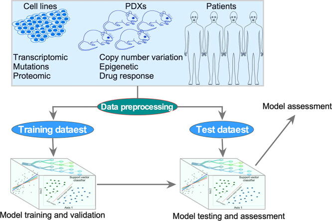
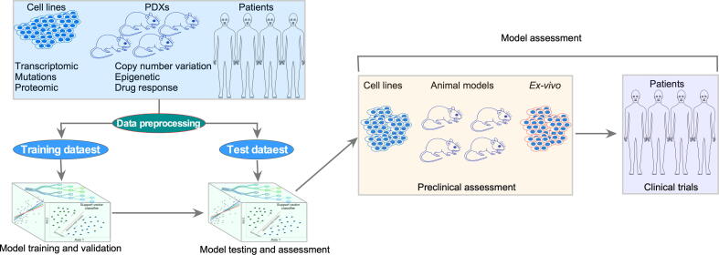
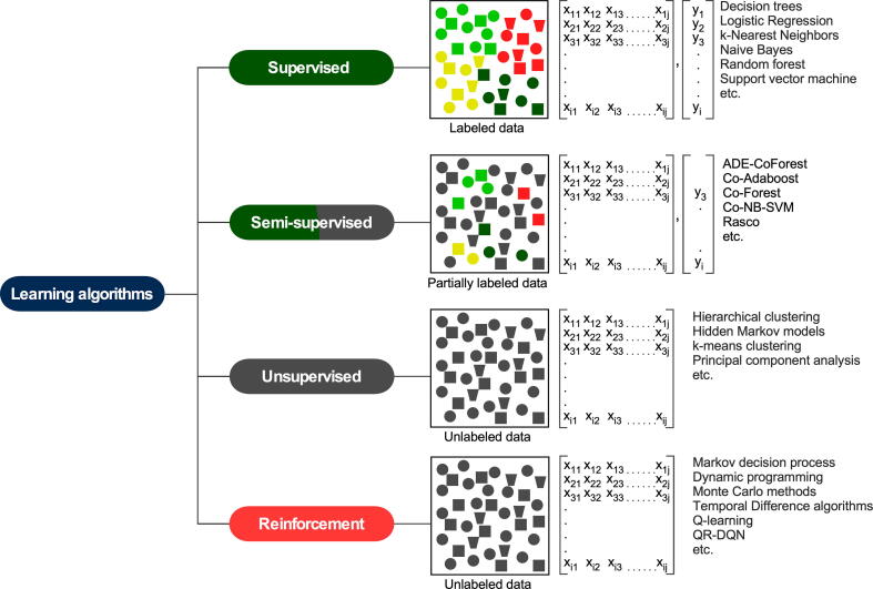
Resistance to therapy remains a major cause of cancer treatment failures, resulting in many cancer-related deaths. Resistance can occur at any time during the treatment, even at the beginning. The current treatment plan is dependent mainly on cancer subtypes and the presence of genetic mutations. Evidently, the presence of a genetic mutation does not always predict the therapeutic response and can vary for different cancer subtypes. Therefore, there is an unmet need for predictive models to match a cancer patient with a specific drug or drug combination. Recent advancements in predictive models using artificial intelligence have shown great promise in preclinical settings. However, despite massive improvements in computational power, building clinically useable models remains challenging due to a lack of clinically meaningful pharmacogenomic data. In this review, we provide an overview of recent advancements in therapeutic response prediction using machine learning, which is the most widely used branch of artificial intelligence. We describe the basics of machine learning algorithms, illustrate their use, and highlight the current challenges in therapy response prediction for clinical practice.

Keywords: Artificial intelligence; Convolutional neural network; Deep learning; Deep neural network; Drug combinations; Drug synergy; Elastic net; Factorization machine; Graph convolutional network; Higher-order factorization machines; Lasso; Matrix factorization; Monotherapy prediction; Ordinary differential equation; Random forests; Restricted Boltzmann machine; Ridge regression; Support vector machines; Variational autoencoder; Visible neural network.

Graphical abstract

Fig. 1

Workflow for ML prediction model development. Pharmacogenomic data from cell lines, patient-derived xenografts (PDXs), and patient materials are ideal for ML model development. Data from different sources are preprocessed and then divided into training (including cross-validation) and test groups. The training dataset is used to build and validate the prediction model, while the test dataset is used for testing the model’s accuracy and precision. To develop a prediction model for clinical use, vigorous preclinical assessment is required that can be performed using cell lines, PDXs, and patient materials that have not been used for model development. Additionally, the efficacy of predicted drugs must be tested for disease-specific preclinical models. Finally, both the model and predicted drug will undergo a clinical trial.

Fig. 2

Schematic representation of different ML algorithms. In a supervised learning model, all data have a known label, while the semi-supervised model can handle partially labeled data. Both unsupervised and reinforcement learning algorithms can handle unlabeled data.

Fig. 3

A comparison of different linear regression algorithms. The sklearn.linear_model from SciKit learn was used to generate example plots using a diabetes dataset provided in SciKit learn. Plots show that by changing the λ value, regression can be regulated such that with a small λ value, all linear regression algorithms provide similar regression. Color code: linear regression – blue, ridge regression – green, lasso – cyan, and elastic net – red. (For interpretation of the references to color in this figure legend, the reader is referred to the web version of this article.)

Fig. 4

Schematic representation of random forest algorithm. The three major steps in the random forest algorithm are bootstrapping, bagging, and aggregation. During bootstrapping, the training dataset is resampled into several small datasets, which are then bagged for the decision tree. The size of the bagged dataset remains the same but bootstrapped decision trees are different from each other. All decision trees make predictions on test data, and in the aggregation step, all predictions are combined for the final prediction. For a classification problem, the final prediction is made by major voting, but for a regression problem, the final prediction uses the mean or median value.

Fig. 5

Support vector machine. (A) In a two-dimensional SVM classification system, the maximum margin classifier is a straight line (red line). Support vectors are the nearest data points from the maximum margin classifier. The distance between support vectors and the maximum margin classifier is denoted as the soft margin. (B) In a two-group, one-dimensional data space, the decision boundary is a point, as shown by the red line. (C) In a two-group one-dimensional data space where the decision boundary cannot be drawn by a point, data are transformed by a kernel function to increase the dimension. (For interpretation of the references to color in this figure legend, the reader is referred to the web version of this article.)

Fig. 6

Deep learning (DL). (A) In a deep neural network (DNN) model, each node of the input data layer is fully connected to the hidden layer nodes. The first hidden layer takes input data, multiplies it by weight, and adds a bias before applying a nonlinear activation function. The second hidden layer takes the first hidden layer as input and so on until it reaches the output layer. (B) In a dropout layer, some nodes are randomly removed. (C) During the convolution, the dimension of input data is reduced using a certain kernel size (in this example, 3x3) and the activation function. Then, features are pulled for further reduction. Finally, pulled features are flattened and applied to a DNN.

Fig. 7

ML algorithms used in the last decade to build monotherapy response prediction. Earlier prediction models were likely developed mainly using classical ML algorithms. Later, the DL algorithms were used mostly to develop the models. The majority of the studies used multi-omics data (mutation, CNV, methylation, and gene expression) collected from large screening studies such as CCLE, GDSC, CTRP, etc. EN – elastic net, RF – random forest, NN – neural network, RR – ridge regression, BM-MKL – Bayesian multitask multi-kernel learning, SVM – support vector machine, LASSO - least absolute shrinkage and selection operator, CNN – convolutional neural network, DNN – deep neural network, AE – autoencoder, VAE – variational autoencoder, MF – matrix factorization, VNN – visual neural network, GCN – graph convolutional network.

Fig. 8

Matrix factorization and factorization machine. (A) In MF, a matrix is decomposed into two lower-dimensional matrices with the same latent factor. The dot product of lower-dimensional matrices is used to reconstitute the new matrix to calculate the loss function. (B) An FM transforms sample and features data to the binary representation and can incorporate additional features.

Fig. 9

Autoencoder and variational autoencoder. (A) The autoencoder determines latent variables by reducing the dimensions during encoding. Then it decodes the data into a similar form using the latent variables. (B) VAE uses a similar process unless the latent variables are replaced by the mean and standard deviation.

References

1. Kourou K., Exarchos T.P., Exarchos K.P., Karamouzis M.V., Fotiadis D.I. Machine learning applications in cancer prognosis and prediction. Comput. Struct. Biotechnol. J. 2015;13:8–17. - PMC - PubMed
1. Sharma A., Rani R. A systematic review of applications of machine learning in cancer prediction and diagnosis. Arch. Comput. Methods Eng. 2021 doi: 10.1007/s11831-021-09556-z. - DOI
1. Hamamoto R., Suvarna K., Yamada M., Kobayashi K., Shinkai N., Miyake M. Application of artificial intelligence technology in oncology: towards the establishment of precision medicine. Cancers (Basel) 2020;12:3532. doi: 10.3390/cancers12123532. - DOI - PMC - PubMed
1. Putora P.M., Baudis M., Beadle B.M., El Naqa I., Giordano F.A., Nicolay N.H. Oncology informatics: status quo and outlook. Oncology. 2020;98(Suppl. 6):329–331. - PMC - PubMed
1. Shimizu H., Nakayama K.I. Artificial intelligence in oncology. Cancer Sci. 2020;111(5):1452–1460. - PMC - PubMed
LinkOut - more resources