Whole-body integration of gene expression and single-cell morphology

Abstract

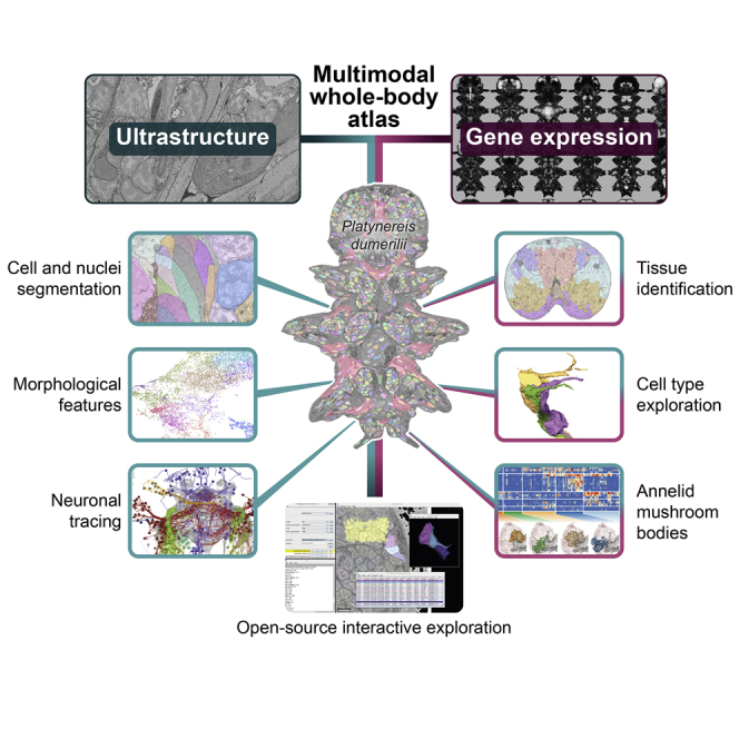
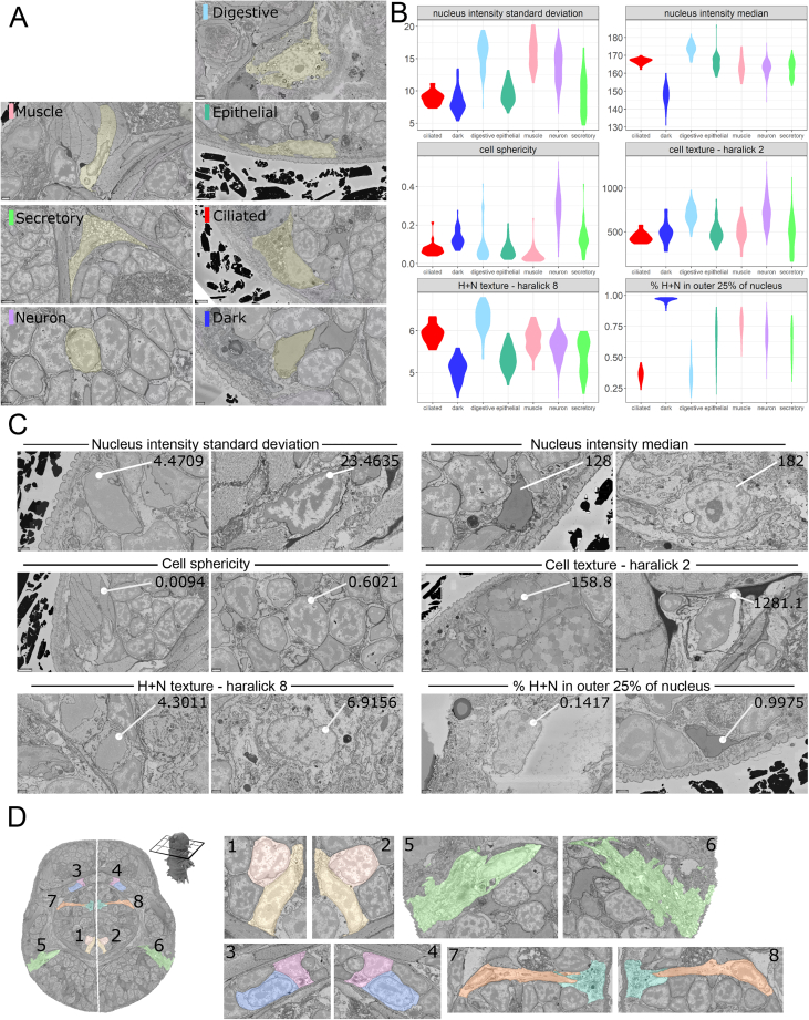
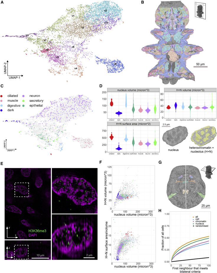
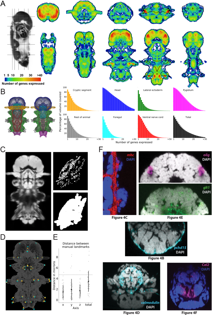
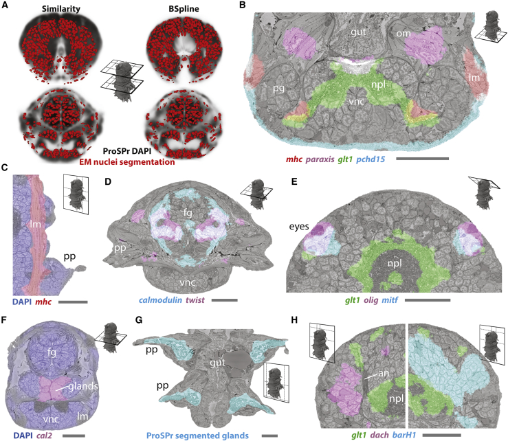
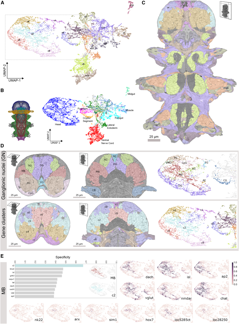
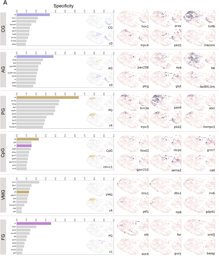
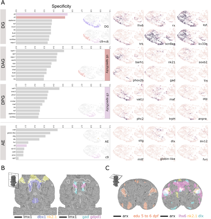
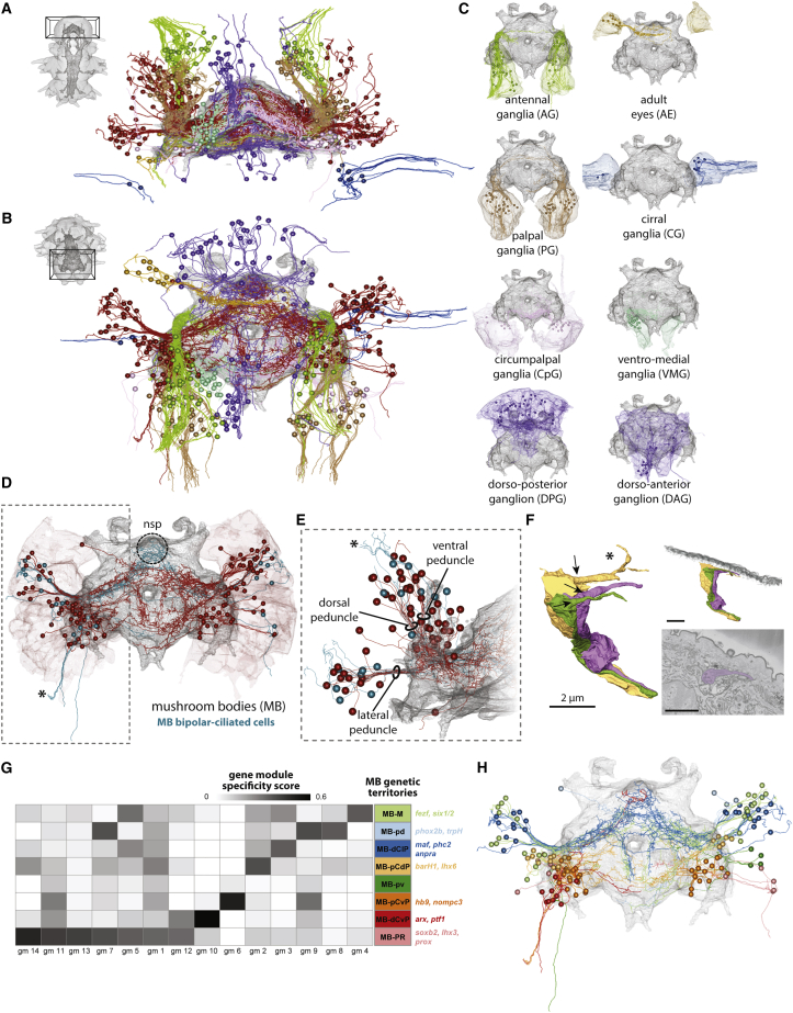
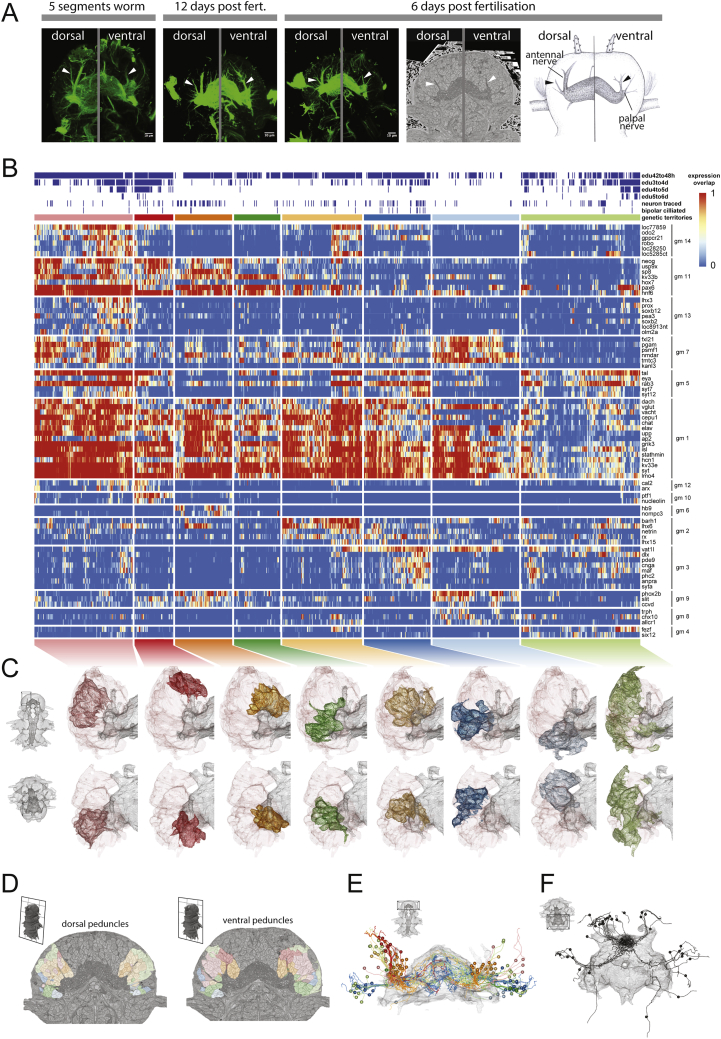
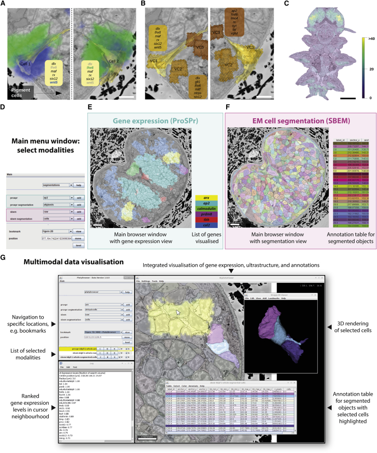
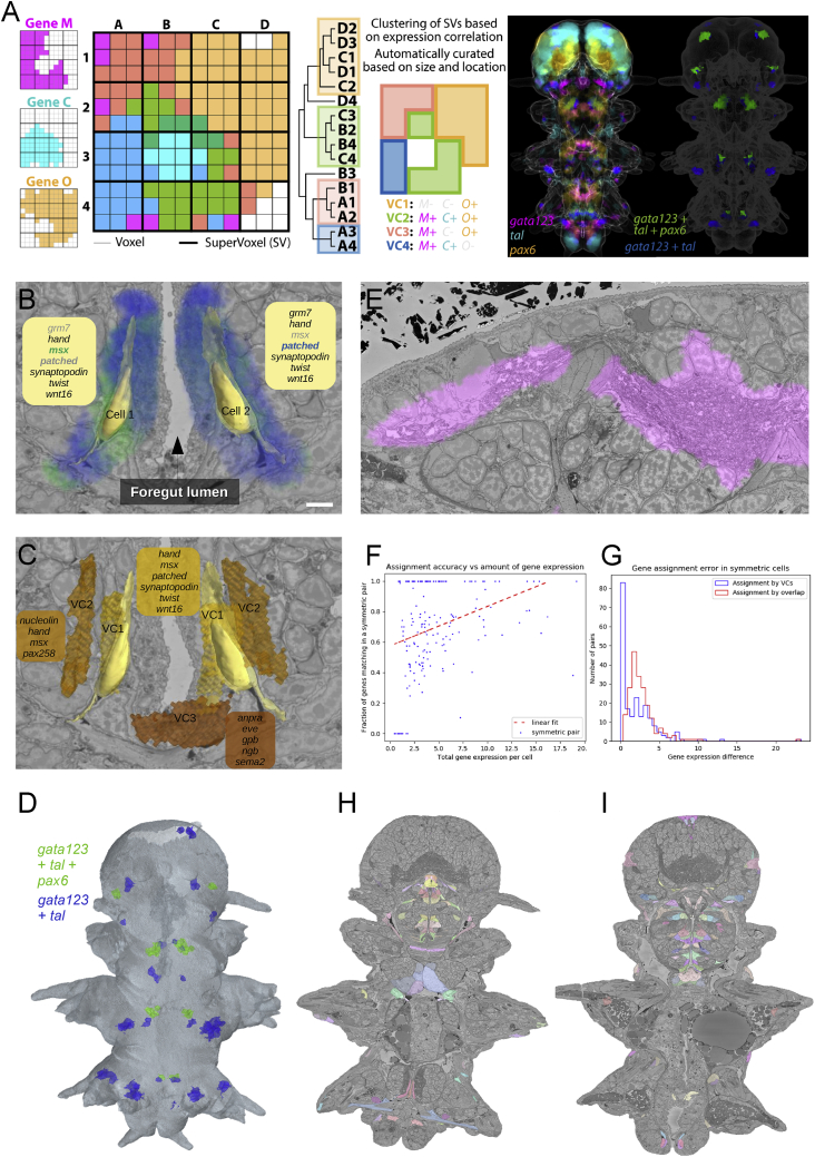
Animal bodies are composed of cell types with unique expression programs that implement their distinct locations, shapes, structures, and functions. Based on these properties, cell types assemble into specific tissues and organs. To systematically explore the link between cell-type-specific gene expression and morphology, we registered an expression atlas to a whole-body electron microscopy volume of the nereid Platynereis dumerilii. Automated segmentation of cells and nuclei identifies major cell classes and establishes a link between gene activation, chromatin topography, and nuclear size. Clustering of segmented cells according to gene expression reveals spatially coherent tissues. In the brain, genetically defined groups of neurons match ganglionic nuclei with coherent projections. Besides interneurons, we uncover sensory-neurosecretory cells in the nereid mushroom bodies, which thus qualify as sensory organs. They furthermore resemble the vertebrate telencephalon by molecular anatomy. We provide an integrated browser as a Fiji plugin for remote exploration of all available multimodal datasets.

Keywords: Platynereis dumerilii; automatic segmentation; cell types; gene expression atlas; image registration; machine learning; multimodal data integration; mushroom bodies; telencephalon; volume electron microscopy.

Graphical abstract

Figure 1

A whole-body serial block-face scanning electron microscopy dataset (A) The SBEM dataset can be observed in all orientations (e.g., transversal plane in top row or the horizontal plane in bottom row; scale bar: 50 μm). (B–E) Fine ultrastructure at native resolution (10 nm pixel-size x/y; scale bars: 2 μm). (B) Epithelial cell, interfacing cuticle, and underlying muscle. Bundles of cytoskeletal filaments (arrowhead) form part of the attachment complex (inset). (C) The adult eye forms a pigment cup composed of pigment cells (PiCs) and rhabdomeric photoreceptors (rPRCs), which extend a distal segment of microvillar projections (mi) for light detection. In the center of the pigment cup is the vitreous body (vb). (D) Longitudinal muscle fibers are cut transversally, displaying cross-sections of the sarcomere as well as of the sarcoplasmic reticulum that contacts the plasma membrane (inset). (E) Cross-section of the distal part of the nephridia, highlighting the autocell junction (arrow). The lumen houses a bundle of motile cilia (with 9+2 microtubules, inset) contributed by each nephridial cell. (B)–(E) are snapshots that can be retrieved via the PlatyBrowser “Bookmark” function. See also Figure S1.

Figure S1

Ultrastructure of different cell types, segmentation validation, and ultrastructure segmentation, related to Figures 1 and 2 A. Ciliated support cells which are part of the nuchal organ in Platynereis. Cytoskeletal fibers (arrowheads) and anchoring points at the junction of the support cell and the underlying muscles are visible (inset) (Scale bar 5 μm). B. Cell of the nephridia which contains a lumen occupied by motile cilia. These cells contain numerous vesicles responsible for various forms of cell transport. A site of endocytosis, identified by the presence of a clathrin-coated pit is highlighted (arrow)(inset) (Scale bar 2 μm). C-F. Orthogonal projections of the image displayed in Figure 1E - scaling factor of 2.5x was applied to the Z plane to get an isotropic render (Scale bars 2 μm). G: Nuclei and cells were annotated by domain experts for 8 slices (4 transversal, 4 horizontal), see leftmost image for example annotations. We used these annotations to find false merge errors, see the two middle images with arrows highlighting the cell membrane not picked up, and false split errors, see two rightmost images with arrows highlighting parts of the cell that were split off, in the automated segmentation. H: The distribution of cilia per cell for the nephridia on both sides is stereotypical as can be seen from the plot. Cilia in a given cross-section of the lumen almost exclusively start off from the same cell, see segmented cilia colored by their cell of origin overlaid on the EM; upper image shows a cross section of the right nephridium, lower image of the left nephridium. I: Chromatin segmentation overlaid on the EM. The dark phase (classical heterochromatin + nucleolus) and the light phase (classical euchromatin) are segmented. Panels A, B and I are available as bookmarks in the PlatyBrowser.

Figure 2

Segmentation of nuclei and cells (A) Horizontal and transverse sections with 3D renderings of cells (left) and nuclei (right). (B) Intertwined epithelial cells shown as EM-overlaid colored segments and 3D renderings. (C) Segmentation of longitudinal muscles highlighted in the bottom rendering, with other muscles rendered in the background. (D) Cross-section of segmented nephridial cell and individually colored cilia (top). (Bottom) 3D rendering of one nephridium with each cilium colored as the cell it belongs to. Bookmarks for views in (B), (C), and (D) (corresponding to Figures 1B, 1D, and 1E) are available in the PlatyBrowser. The scale bar in (A) corresponds to 50 μm and in (B)–(D) to 2 μm. See also Figure S1.

Figure S2

Morphological analysis of cell types and bilateral pair analysis, related to Figure 3 A: Examples of manually identified cell types from the EM dataset. B: More examples of morphological features that vary between cell types (extension of Figure 3D) C: Example images from the EM dataset of cells with low and high values for a selection of morphological features. The morphological features shown here are the same as in B. D: Higher resolution images of the example bilateral pairs from Figure 3G. Numbers indicate the location of the images in the overview on the left. Panels A, C and D are available as bookmarks in the PlatyBrowser.

Figure 3

Morphological clustering of segmented cells (A) UMAP of all cells based on morphological features, colored by morphological clusters (c0–c10). (B) Morphological clusters mapped on an EM section. (C) 978 manually identified cells mapped on UMAP. (D) Violin plots comparing 3 morphological features between the manually identified cell classes. Bottom right: example nucleus with chromatin segmentation. (E) Super-resolution 3D structured illumination microscopy of Platynereis nuclei. Immuno-labeled histone H3K36me3 (green) indicates active gene bodies on the surfaces of chromatin domains labeled with 4’, 6-diamidino-2-phenylindole (DAPI) (magenta). Upper panel shows lateral, lower panel orthogonal cross-section of a 3D image stack. (F) Scatterplots relating morphological features between all cells with manually identified cells labeled as in (C) and (D). (G) Example section with 7 bilateral cell pairs (midline in white). (H) Fraction of cells finding potential bilateral partners within a certain number of morphological neighbors (see STAR Methods). Legend refers to the features used. (B) and (G) are available as bookmarks in the PlatyBrowser. See also Figure S2.

Figure S3

ProSPr expression atlas gene coverage and registration to the EM, related to Figure 4 A: Genetic coverage throughout the animal. Transversal and horizontal sections color-coded based on the amount of expression information, in gene number, for every pixel. Black contours outline the DAPI-based reference, thresholded for illustration purposes. B: Quantification of gene coverage by animal region. Animal regions are colored as indicated in the 3D views. Histograms represent the percentage of volume containing signal for the number of genes indicated in the x axis. (C): Exemplary single planes of the image data stacks, which were used as input to the registration. Left: DAPI: Average DAPI signal of 153 images from the ProSPr atlas. Top-right: EM-Nuclei: Mask of segmented nuclei of the EM individual. Bottom-right: EM-Mask: Binary mask, created by dilation and binarisation of the EM-Nuclei image. The EM-Mask was used to restrict the elastix optimization algorithm to relevant parts of the image. (D): three-dimensional visualization of the overlay after final registration (see methods) between the 43 manually selected landmarks in both datasets. Landmarks in the SBEM dataset are plotted in orange, and landmarks in the ProSPr atlas are plotted in cyan. Spheres have a diameter of 5 μm. Plotted in ProSPr space. The gray outline is an arbitrary mask extracted from the DAPI signal. (E): quantification of the distance between the 43 landmarks in each axis (ProSPr atlas space: ‘x’ corresponds to medio-lateral, ‘y’ to anterior-posterior, and ‘z’ to dorso-ventral axis), and in total. Horizontal dashed line represents the average cell diameter. (F): confocal slices of individual whole-mount in situ hybridizations showing raw gene expression for some genes shown in Figure 4.

Figure 4

Registration of EM volume and ProSPr gene expression atlas (A) Comparison between similarity and BSpline transform, illustrated with two transversal slices. ProSPr DAPI reference (gray tones) with overlaid segmented EM nuclei (red). Cross-sections through head (top) and foregut (bottom). (B–H) Examples of ProSPr atlas-volume EM overlay. Segmented glands (G) were extracted from the ProSPr dataset using autofluorescence. Scale bar is 25 μm in all images. Raw data for some genes are shown in Figure S3F. (B)–(H) bookmarks are available in the PlatyBrowser. an, antennal nerve; fg, foregut; lm, longitudinal muscles; npl, neuropil; om, oblique muscles; pg, peripheral ganglia; pp, parapodia; vnc, ventral nerve cord. See also Figure S3.

Figure 5

Correlation of gene expression with morphologically defined tissues (A) UMAP of all cells based on the expression of 201 genes. Points are colored by gene expression clusters (c0–c14). Gray rectangle, part of the UMAP shown in (D) and (E). (B) Main body parts in 6-dpf Platynereis with matching colors between animal regions and UMAP. (C) Gene clusters mapped onto an EM section. (D) Comparison of anatomically (top) and genetically (bottom) defined units mapped on transversal (left) and horizontal (middle) head section and UMAP (right). (E) F1 specificity score for mushroom bodies (MBs) and the 10 top scoring genes and clusters (see STAR Methods). The MB, cluster c2, and the expression of 12 genes mapped onto the head region of the UMAP are shown. See Figure S4 for specificity of the remaining ganglionic nuclei (GN). For (C) and the EM overlays of (D), bookmarks are available in the PlatyBrowser. AEs, adult eyes; AG, antennal GN; CG, cirral GN; CpG, circumpalpal GN; DG, dorsal GN; FG, frontal GN; MBs, mushroom bodies; PG, palpal GN; VMG, ventro-medial GN. See also Figure S4.

Figure S4

Specificity of gene clusters and individual genes for head ganglia, related to Figure 5 A: Comparison of specificity of gene clusters and individual genes for the head ganglia. Left column – graphs of top 10 scoring genes (gray bars) or gene clusters (colored bars) by F1 specificity score (see methods). Inset– zooms of the head region of the UMAP from Figure 5A colored by ganglia (top) and top scoring genetic clusters (bottom). Right column - gene expression overlap value (0-1, same scale as in Figure 5E) for example genes. Note: here we show only the head region of the UMAPs, for easier comparison, but some genes and gene clusters have expression domains outside of the head which contribute to their lower specificity scores. loc8913nt corresponds to the ionotropic glutamate receptor igluR. Other genes starting with ‘loc’ are GPCR-related but without clearly identified homologs. Abbreviations: AG, antennal ganglia; CG, cirral ganglia; CpG, circumpalpal ganglia; FG, frontal ganglion; VMG, ventro-medial ganglia. B: Frontal cross-section of the ventral brain illustrating co-expression of genes in the ventromedial ganglion. The expression region of lmx1 is illustrated with white contours. C: Dorsal cross-section of the brain illustrating one of the proliferative regions of the mushroom bodies and the specific co-expression of transcription factors. The expression region of arx is illustrated with white contours. Panels B and C are available as bookmarks in the PlatyBrowser. Abbreviations: AE, adult eyes; DG, dorsal ganglion; DAG, dorso-anterior ganglion; DPG, dorso-posterior ganglion.

Figure S4

Specificity of gene clusters and individual genes for head ganglia, related to Figure 5 A: Comparison of specificity of gene clusters and individual genes for the head ganglia. Left column – graphs of top 10 scoring genes (gray bars) or gene clusters (colored bars) by F1 specificity score (see methods). Inset– zooms of the head region of the UMAP from Figure 5A colored by ganglia (top) and top scoring genetic clusters (bottom). Right column - gene expression overlap value (0-1, same scale as in Figure 5E) for example genes. Note: here we show only the head region of the UMAPs, for easier comparison, but some genes and gene clusters have expression domains outside of the head which contribute to their lower specificity scores. loc8913nt corresponds to the ionotropic glutamate receptor igluR. Other genes starting with ‘loc’ are GPCR-related but without clearly identified homologs. Abbreviations: AG, antennal ganglia; CG, cirral ganglia; CpG, circumpalpal ganglia; FG, frontal ganglion; VMG, ventro-medial ganglia. B: Frontal cross-section of the ventral brain illustrating co-expression of genes in the ventromedial ganglion. The expression region of lmx1 is illustrated with white contours. C: Dorsal cross-section of the brain illustrating one of the proliferative regions of the mushroom bodies and the specific co-expression of transcription factors. The expression region of arx is illustrated with white contours. Panels B and C are available as bookmarks in the PlatyBrowser. Abbreviations: AE, adult eyes; DG, dorsal ganglion; DAG, dorso-anterior ganglion; DPG, dorso-posterior ganglion.

Figure 6

Expression profile and neural projections of head ganglia and mushroom bodies (A) Ventral 3D visualization of all neurons reconstructed in this study, with cell bodies represented as spheres and cellular projections skeletonized. Neuropil is represented as a gray mesh, and neurons are colored as their GN in Figure 5. (B) Same as in (A) from an anterior-dorsal view. (C) Anterior-dorsal 3D views of individual GN illustrating the volume of all constituting cells and the traced cells. (D) Same as in (C) for the MB, highlighting bipolar cells in cyan. (E) Frontal view of the right mushroom body (dotted box in D). Rings indicate the dorsal and ventral peduncles of the mushroom bodies (see Figure S5). (F) Dense reconstruction of sensory endings of 3 colored bipolar cells (asterisks in D and E). Arrows indicate the base of the sensory cilia. On the top right, same rendering from a different perspective to show that the cilia remain below the cuticle, rendered in gray. On the bottom right, EM image for one of the cilia. (F) is available as a bookmark in the PlatyBrowser. (G) Heatmap showing the specificity score of gene modules (gm) for the different genetic territories in the MB (see Figure S5 and STAR Methods). (H) MB traced cells colored by the genetic territory (G and Figures S5B–S5E) they belong to. MB-M, mantle; MB-pd, posterior-dorsal; MB-dClP, distal calyx lateral peduncle; MB-pCdP, proximal calyx dorsal peduncle; MB-pv, posterior-ventral; MB-pCvP, proximal calyx ventral peduncle; MB-dCvP, distal calyx ventral peduncle; MB-PR, progenitor region. See also Figure S5.

Figure S5

Anatomico-molecular analysis of the mushroom bodies at 6 dpf, related to Figure 6 A: Illustration of the identification of mushroom bodies peduncles from the juvenile worm, where both the cellular and neuropil structures are clearly recognizable, to the 6 dpf Platynereis. The first three panels are maximum projection images of confocal stacks, obtained from acetylated tubulin immunostainings. The fourth panel is obtained from the EM dataset. The fifth panel is a simplified illustration of the relevant structures shown in the rest of the panels. All panels are composed of two views at different dorso-ventral locations to highlight the dorsal and ventral peduncles, indicated with arrowheads. B: Heatmap for all cells that constitute the mushroom bodies (MB) ganglia. Only the 75 most variable genes are shown. Cells are grouped into clusters (genetic territories; see methods), and hierarchically ordered within each cluster. The order of the MB clusters in the heatmap is established using hierarchical clustering of cluster expression means. Rows are ordered by gene modules as in Figure 6G. Genes within each module are ordered by specificity values of each gene (see methods). On the top of the heatmap, blue indicates cells positive for proliferative EdU stainings done at distinct developmental stages, as well as cells that are traced, and those found to show bipolar projections (sensory endings). Genes starting with ‘loc’ are GPCR-related but without clearly identified homologs. C. 3D views of the MB genetic territories, each color-coded according to their colors in the heatmap. The neuropil is plotted in gray, and the mesh of the entire mushroom body ganglion is plotted as well for reference. The top row shows the ventral view and the bottom row the anterio-dorsal view. The regions shown are specified in the models shown in the left. D. EM slices at the level of the two peduncles. E. Frontal 3D view of the cells traced for the mushroom bodies ganglia (see Figure 6G). In D and E, cells are color-coded according to which MB genetic territory they belong to. F. Anterio-dorsal 3D view of the traced dark cells (see section on cell morphology; Figures 3 and S2).

Figure 7

Virtual cells and the PlatyBrowser (A) Assignment by gene overlap illustrated for lhx6 and wnt5 (blue and green), for a pair of bilateral cells. In boxes, assigned genes show >50% overlap. Genes in light gray fail to be assigned. Scale bars: 5 μm. (B) Assignment to virtual cells for the same cells as in (A). (C) Number of assigned genes per segmented cells after virtual cell assignment (scale bar: 50 μm). For (A)–(C), bookmarks are available in the PlatyBrowser. (D) User interface to select image sources, change their appearance, and navigate to specific locations in the animal. (E) BigDataViewer, showing the SBEM image in a region of the adult head, with the ProSPr signal for six different genes. (F) BigDataViewer of the same section as in (B), now displaying the cellular segmentation. (G) Screenshot of the PlatyBrowser illustrating the integration of modalities and additional functionalities: the expression of gene arx is shown in yellow; three segmented neurons are shown next to it; and annotation table below with highlighted rows that correspond to selected objects. The 3D Viewer window shows a rendering of the selected cells; the colors for a given object are identical in the 2D Viewer overlay, 3D rendering, and table. Below the main menu, the log window shows a ranked list of gene expression where the mouse cursor is positioned (white arrow). See also Figure S6.

Figure S6

Gene expression assignment, related to Figure 7 A: Generation of Virtual Cells. On the left, hypothetical spatial expression of three different genes in a 12 × 12 voxel array. In the matrices, thin lines demarcate the voxels and dark ones supervoxels. Voxel colors indicate all possible combinations of expressions (e.g., gene C + gene M in dark blue). The hierarchical tree illustrates the process of clustering supervoxels based on expression information, which renders groups of supervoxels called Virtual Cells (VCs), that are then automatically curated based on size and spatial location. The VCs are visualized spatially on the matrix next to the tree with their expression information. On the right, illustration of this procedure with real data. Three genes are shown on a projection image of the full dataset using similar coloring for the co-expression as in the example on the left. Next to it, the coloring of VCs showing a specific expression pattern (2 examples). Note that each of these groups is composed of many VCs but all have the same coloring for illustration purposes. B-C: The difference between assignment by overlap and assignment to genetically nearest Virtual Cell. (B): Assignment by overlap: biological variability and registration error resulted in slight asymmetry of the gene expression volumes of the genes patched and msx (blue and green). Gene lists correspond to genes that would be assigned as expressed in the cell if the assignment was done by volume overlap (regular print for genes with > 50% overlap, light gray font for the rest). With a fairly conservative 50% overlap threshold, the resulting assignment for the bilaterally symmetric cells would be different (scale bars: 5 μm). (C): Assignment to Virtual Cells: for each segmented cell the neighboring Virtual Cell that has the smallest genetic difference is assigned. This results in a consistent assignment of denoised genetic profiles (scale bars: 5 μm). (D): The assignment of the Virtual Cells shown on panel A to the segmented cells. The cells in blue were assigned Virtual Cells that express genes gata123 and tal, the ones in green - genes gata123, tal, and pax6. (E): ‘Gene leaking’ of glt1 (glutamate receptor). While the true expression is confined to the neuropil, the bordering regions such as neural somas, muscles and epithelial cells also show a high level of expression, originating from sample variability and limited registration accuracy. F: Dependency of the assignment accuracy on the total level of gene expression in a cell (the fractions of gene expression for each gene summed up). The assignment performed better for the cells in gene rich areas. (G): Assignment errors in the symmetric cells pairs for the Virtual Cells assignment and assignment by overlap. Assignment error is defined as the absolute difference in gene expressions assigned to the cells of a symmetric pair. H-I: Examples of symmetric cell pairs – cells with similar mirror location and morphology, supposedly representing the same cell type and expressing the same genes. For panels B,C,H and I bookmarks are available in the PlatyBrowser.

References

1. Achim K., Eling N., Vergara H.M., Bertucci P.Y., Musser J., Vopalensky P., Brunet T., Collier P., Benes V., Marioni J.C., Arendt D. Whole-body single-cell sequencing reveals transcriptional domains in the annelid larval body. Mol. Biol. Evol. 2018;35:1047–1062. - PMC - PubMed
1. Altun Z.F., Herndon L.A., Wolkow C.A., Crocker C., Lints R., Hall D.H. 2002. WormAtlas.http://www.wormatlas.org
1. Anderson J.R., Jones B.W., Watt C.B., Shaw M.V., Yang J.-H., Demill D., Lauritzen J.S., Lin Y., Rapp K.D., Mastronarde D. Exploring the retinal connectome. Mol. Vis. 2011;17:355–379. - PMC - PubMed
1. Arendt D., Musser J.M., Baker C.V.H., Bergman A., Cepko C., Erwin D.H., Pavlicev M., Schlosser G., Widder S., Laubichler M.D., Wagner G.P. The origin and evolution of cell types. Nat. Rev. Genet. 2016;17:744–757. - PubMed
1. Arganda-Carreras I., Sorzano C.O.S., Marabini R., Carazo J.M., Ortiz-de-Solorzano C., Kybic J. In: Beichel R.R., Sonka M., editors. Springer Berlin Heidelberg; 2006. Consistent and elastic registration of histological sections using vector-spline regularization; pp. 85–95. (Computer Vision Approaches to Medical Image Analysis).
Publication types