Plasma Turbulence at Comet 67P/Churyumov-Gerasimenko: Rosetta Observations

Abstract

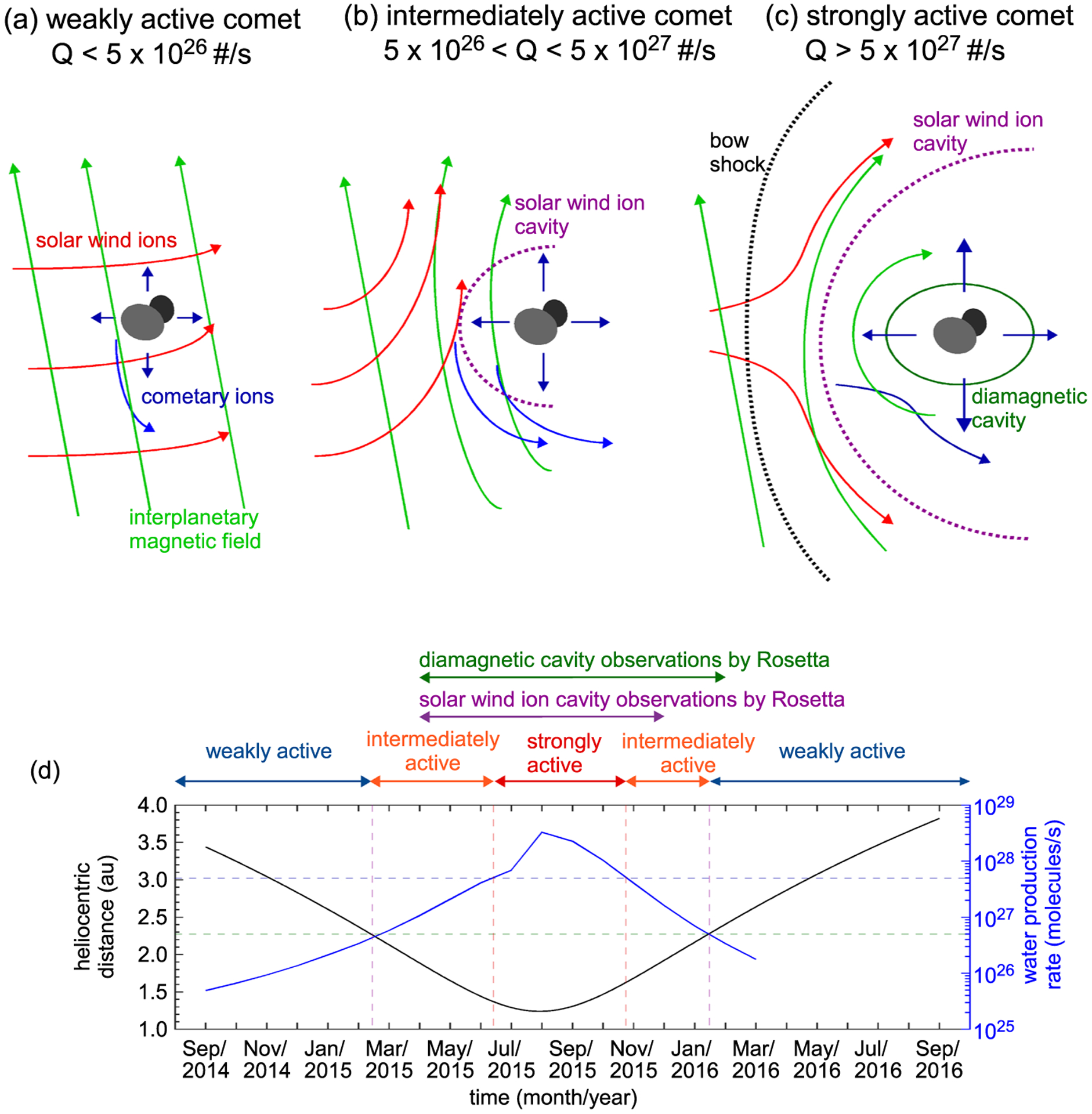
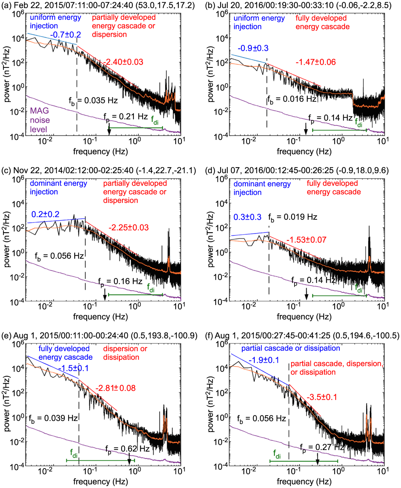
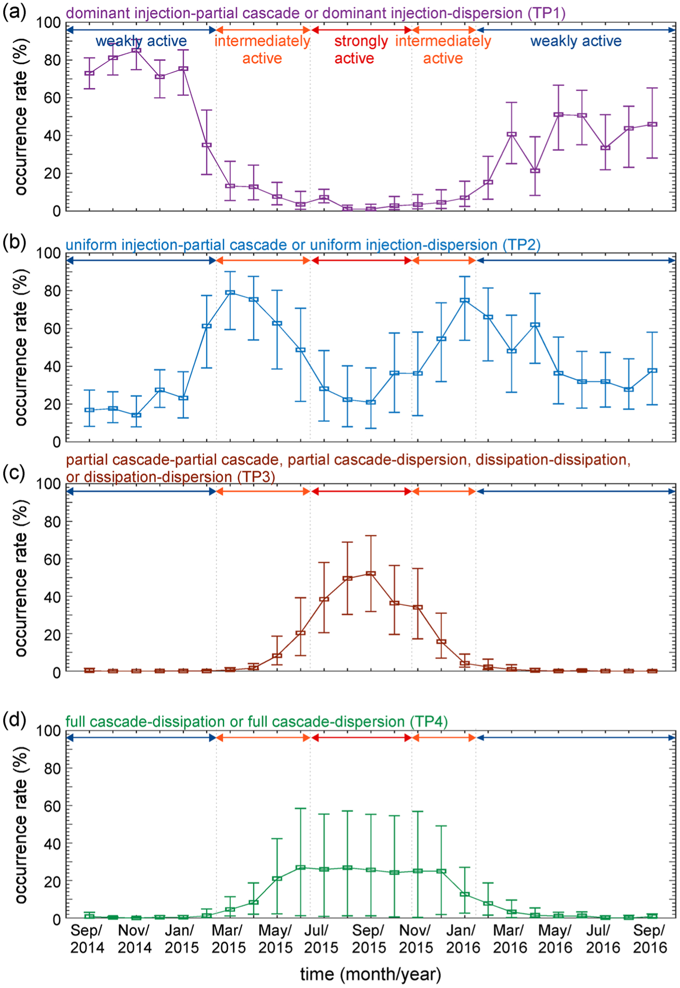
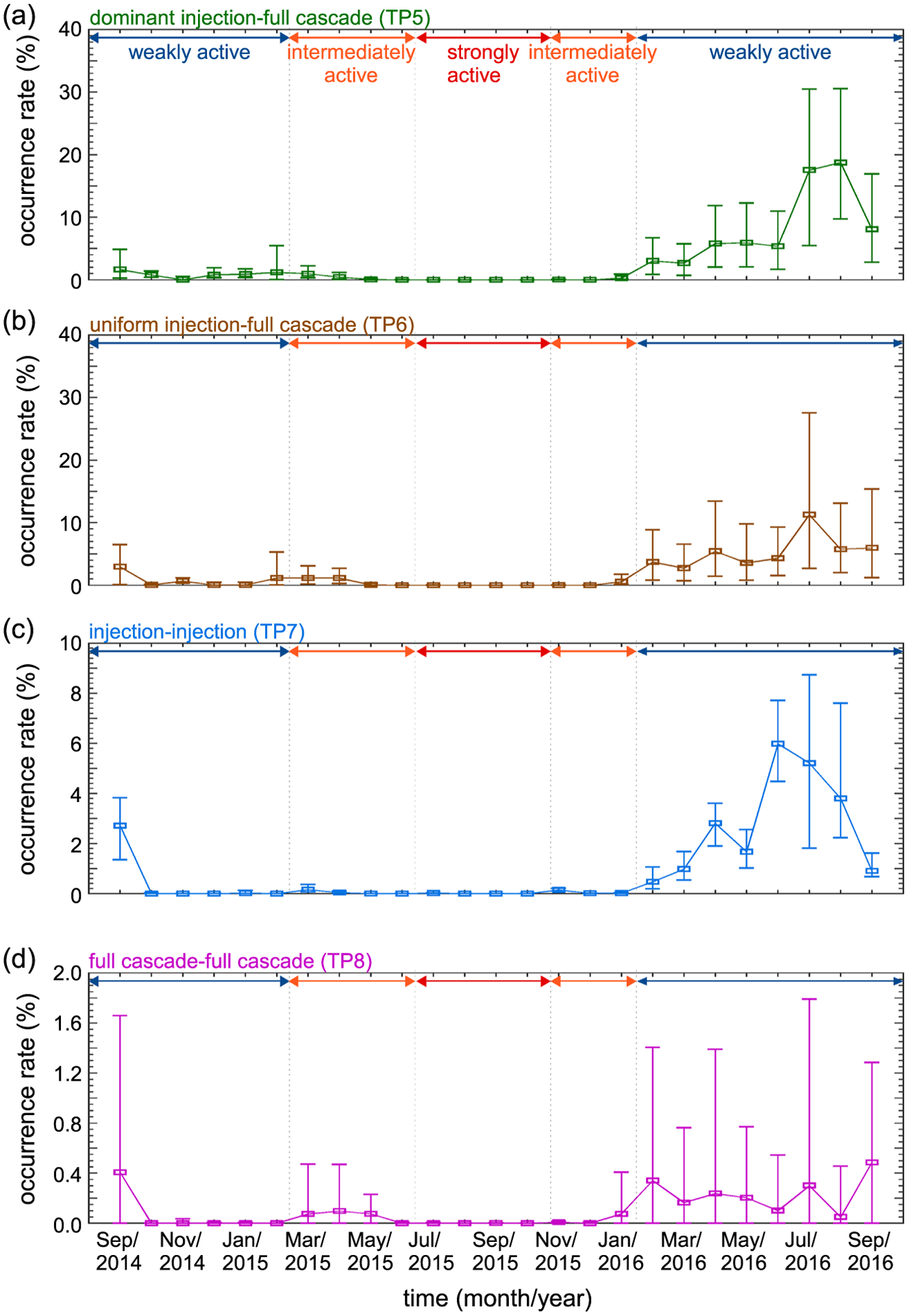
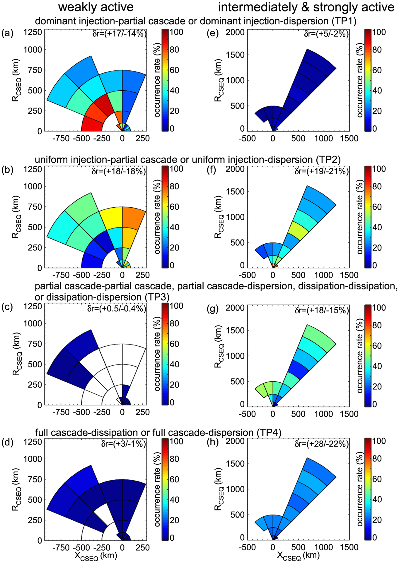
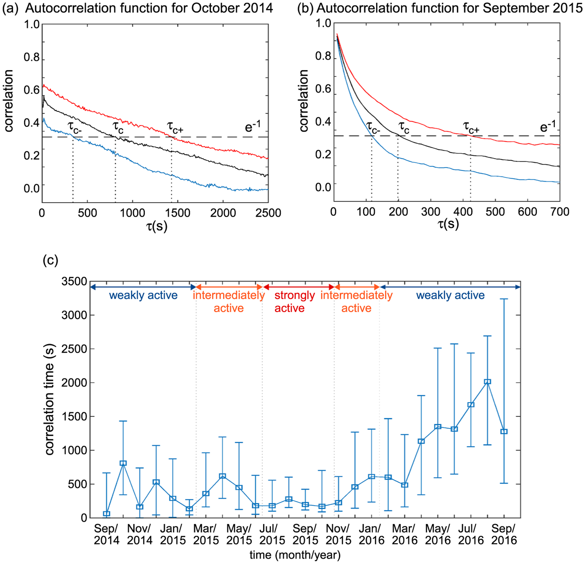
We perform a power spectral analysis of magnetic field fluctuations measured by the Rosetta spacecraft's magnetometer at comet 67P/Churyumov-Gerasimenko. We interpret the power spectral signatures in terms of plasma turbulent processes and discover that different turbulent processes are prominent during different active phases of the comet. During the weakly active phase of the comet, dominant injection is prominent at low frequencies near 10^-2 Hz, while partial energy cascade or dispersion is prominent at high frequencies near 10^-1 Hz. During the intermediately active phase, uniform injection is prominent at low frequencies, while partial energy cascade or dispersion is prominent at high frequencies. During the strongly active phase of the comet, we find that partial energy cascade or dissipation is dominant at low frequencies, while partial energy cascade, dissipation, or dispersion is dominant at high frequencies. We infer that the temporal variations of the turbulent processes occur due to the evolution of the plasma environment of the comet as it orbits the Sun.

Figure 1.

The plasma environment of a comet as it transitions from a weakly active comet to a strongly active comet is shown in (a–c). This figure is based on Figure 1.1 of Götz et al. (2019). Heliocentric distance of comet 67P from September 2014 to September 2016 is shown in (d). The empirical fits for water production rate Q determined by Hansen et al. (2016) are also shown in (d).

Figure 2.

Six different power spectra of magnetic field fluctuations observed at comet 67P, which depict six different combinations of turbulent processes, are shown in (a–f). The frequency at which a sharp transition of the spectral indices occurs is indicated by f b, which is the spectral break frequency. The local proton gyrofrequency is indicated by f p. The time interval associated with each power spectrum is provided above each panel. The mean solar equatorial frame (CSEQ) coordinates for the spacecraft are also provided in kilometers, within brackets above each panel.

Figure 3.

Procedure for determining the spectral break frequency for a power spectrum is depicted in (a–c).

Figure 4.

Median spectral break frequencies and median low- and high-frequency spectral indices for each month with their quartiles are shown in (a) and (b).

Figure 5.

Occurrence rates for TP1–TP4 turbulent processes from September 2014 to September 2016 are shown in (a–d).

Figure 6.

Occurrence rates for TP5–TP8 turbulent processes from September 2014 to September 2016 are shown in (a–d).

Figure 7.

Spatial occurrence rate maps for TP1–TP4 turbulent processes during the weakly active phase are shown in (a–d). Spatial occurrence rate maps for TP1–TP4 turbulent processes during the intermediately and strongly active phases are shown in (e–h). In these figures, $R_{\mathit{\text{CSEQ}}}=\sqrt{Y_{\mathit{\text{CSEQ}}}^2+Z_{\mathit{\text{CSEQ}}}^2}$ is the radial distance from the comet. X_CSEQ > 0 side is the sunward side of the comet or the dayside. δr in each panel indicates the uncertainty of the occurrence rates.

Figure 8.

Median and quartiles of autocorrelation function for magnetic field for two representative times are shown in (a) and (b). Median correlation times and their uncertainties for each month from September 2014 to September 2016 are shown in (c).

References

-
- Alexandrova O, Carbone V, Veltri P, & Sorriso-Valvo L (2008). Small-scale energy cascade of the solar wind turbulence. The Astrophysical Journal, 674, 1153–1157. 10.1086/524056 - DOI
- Alexandrova O, Lacombe C, Mangeney A, Grappin R, & Maksimovic M (2012). Solar wind turbulent spectrum at plasma kinetic scales. The Astrophysical Journal, 760, 121. 10.1088/0004-637X/760/2/121 - DOI
- Behar E, Lindkvist J, Nilsson H, Holmström M, Stenberg-Wieser G, Ramstad R, & Götz C (2016). Mass-loading of the solar wind at 67P/Churyumov-Gerasimenko: Observations and modeling. Astronomy & Astrophysics, 596, A42. 10.1051/0004-6361/201628797 - DOI
- Behar E, Nilsson H, Alho M, Goetz C, & Tsurutani B (2017). The birth and growth of a solar wind cavity around a comet—Rosetta observations. Monthly Notices of the Royal Astronomical Society, 469, S396–S403. 10.1093/mnras/stx1871 - DOI
- Behar E, Nilsson H, Stenberg-Wieser G, Nemeth Z, Broiles TW, & Richter I (2016). Mass loading at 67P/Churyumov-Gerasimenko: A case study. Geophysical Research Letters, 43, 1411–1418. 10.1002/2015GL067436 - DOI
Grants and funding
LinkOut - more resources
Full Text Sources