Vitrification and Nanowarming of Kidneys

Abstract

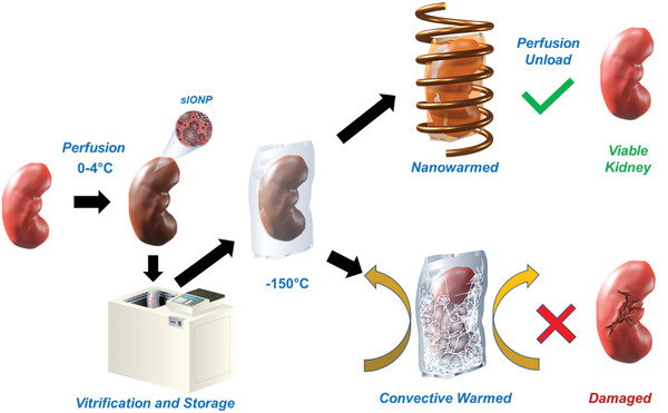
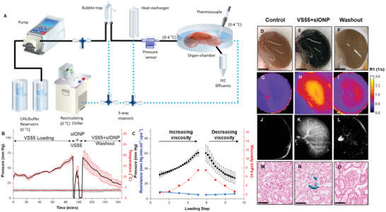
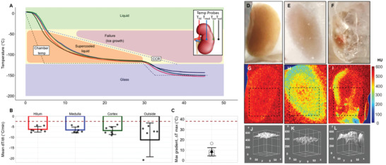
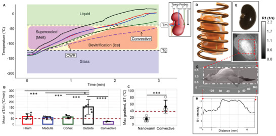
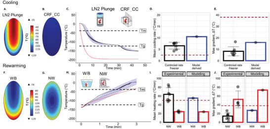
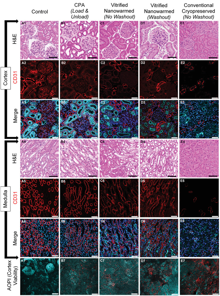
Vitrification can dramatically increase the storage of viable biomaterials in the cryogenic state for years. Unfortunately, vitrified systems ≥3 mL like large tissues and organs, cannot currently be rewarmed sufficiently rapidly or uniformly by convective approaches to avoid ice crystallization or cracking failures. A new volumetric rewarming technology entitled "nanowarming" addresses this problem by using radiofrequency excited iron oxide nanoparticles to rewarm vitrified systems rapidly and uniformly. Here, for the first time, successful recovery of a rat kidney from the vitrified state using nanowarming, is shown. First, kidneys are perfused via the renal artery with a cryoprotective cocktail (CPA) and silica-coated iron oxide nanoparticles (sIONPs). After cooling at -40 °C min^-1 in a controlled rate freezer, microcomputed tomography (µCT) imaging is used to verify the distribution of the sIONPs and the vitrified state of the kidneys. By applying a radiofrequency field to excite the distributed sIONPs, the vitrified kidneys are nanowarmed at a mean rate of 63.7 °C min^-1 . Experiments and modeling show the avoidance of both ice crystallization and cracking during these processes. Histology and confocal imaging show that nanowarmed kidneys are dramatically better than convective rewarming controls. This work suggests that kidney nanowarming holds tremendous promise for transplantation.

Keywords: cryopreservation; iron oxide nanoparticles; kidney; perfusion; radiofrequency warming; vitrification.

Figure 1

Schematic flow of kidney nanowarming. The kidney is hypothermically (0–4 °C) perfused with CPA (VS55) and sIONPs through the renal artery, then immersed in a cryobag containing VS55+sIONP and cooled rapidly to a vitrified state at −150 °C in a controlled rate freezer (CRF). During rewarming, convective warming in air or water‐bath will result in ice crystallization due to insufficient warming rates and/or cracking from thermomechanical gradients, thus damaging the kidney. In contrast, nanowarming of the kidney, using an RF magnetic field, results in rapid and uniform heating, minimizing cryopreservation damage that results in recovery similar to CPA load and unload only controls.

Figure 2

Hypothermic perfusion loading and unloading of rat kidneys with VS55+sIONPs. A) Schematic layout of the hypothermic perfusion circuit. The cold CPA (0–4 °C) is perfused using a peristaltic pump through a bubble trap and a heat exchanger before entry into the renal artery. Pressure and temperature sensors record the arterial pressure and chamber temperature, respectively, throughout the experiment. A circulating chiller is used to cool the bubble trap, heat exchanger, and organ chamber. B) Mean arterial pressure and chamber temperature variation over time during hypothermic perfusion loading and unloading of a rat kidney with VS55 and sIONPs. Error bars indicate the standard error (SEM) for n = 4 rat kidneys. The loading steps were Euro Collins (EC), 18.75%, 25%, 50%, 75%, and 100% v/v (8.4 m) VS55 and the wash out steps were 75%, 50%, 25% VS55 (v/v), and EC (Table S2, Supporting Information); no osmotic buffering was used during washout. C) Variation of peak pressure over the loading and unloading steps correlates with increase and decrease in viscosity of the perfusate, as VS55 concentration is increased during loading and decreased during washout. At each loading step, there is an overall increase in pressure due to the increase in viscosity overlapping with a transient reduction in pressure due to the vascular osmotic response to the increased concentration (osmotic vasodilation—Figure 2B; Figure S2, Supporting Information); As a net result, calculated resistance, R (blue points) actually decreases as viscosity increases; shaded blue region indicates 95% confidence interval of a linear fit of R versus time (loading steps). R is only calculated for VS55 loading and washout, not during sIONP loading. D–F) Gross images of a control, VS55+sIONP loaded and washed‐out kidney, respectively. Scale bar is 0.5 cm. G–I) MR images depicting the distribution of sIONPs, as based on the water relaxation rate constant (R1), of a control, VS55+sIONP loaded and washed‐out kidney, respectively. J–L) X‐ray µCT images of a control, VS55+sIONP loaded and washed‐out kidney, respectively, showing spatial resolution of sIONPs in the kidney vasculature. M–O) Prussian blue staining, to show Fe deposition in a control, VS55+sIONP loaded and washed‐out kidney, respectively. Fe localization is seen in the glomeruli of VS55+sIONP loaded kidneys. Washed out kidneys show clear glomeruli. Scale bar is 150 µm for histology images.

Figure 3

Vitrification success and failure in VS55 loaded kidneys. A) Temperature versus time (T vs t) plot during cooling of a kidney for vitrification. Cooling was performed in a bag‐setup (Methods, Figure S6, Supporting Information) in a controlled rate freezer (CRF). As shown in the inset, fiber optic temperature probes were placed in the hilum, medulla, cortex and outside the kidney (inside the bag) to measure temperature distribution during cooling. B) Mean, SEM, and scatter plot of cooling rates measured at each probe location, for n = 7 kidneys, relative to CCR of VS55 (dotted line). Mean cooling rates at all probe locations were faster than the CCR for VS55, suggesting no ice crystallization. C) Mean, SEM, and scatter plot of maximum gradient ∆T in the glassy state for n = 7 kidneys. These are well below the dotted line indicating the maximum stress‐to‐fracture threshold of ∆T _max (38 °C) for VS55. D–F) Gross images of a vitrified, frozen, and a cracked kidney, respectively. G–I) X‐ray µCT of a vitrified, frozen and cracked kidney, respectively. X‐ray attenuation differences between cases, expressed in Hounsfield Units (HU), are used to detect amorphous (vitrified) versus frozen regions in the kidney and abrupt/sharp X‐ray attenuation changes, indicating cracks. J–L) 3D surface histogram plots for dotted square regions in Figure 3G–I, respectively, indicate spatial X‐ray attenuation differences in vitrified, frozen, and cracked kidneys, within a given plane.

Figure 4

Rewarming of VS55 + sIONP loaded and vitrified rat kidneys. A) Temperature versus time (T vs t) plot during nanowarming and convective warming (negative control) of a kidney from the vitrified state. Nanowarming was performed by placing the vitrified kidney in an RF solenoid coil (D) and rewarming at 180 kHz and 63 kA m⁻¹ alternating magnetic field. As shown in the inset in (A), fiber optic temperature probes were placed in the hilum, medulla, cortex and outside the kidney (fixed inside the vitrified bag) to measure temperature distribution during rewarming. Convective rewarming was performed in a water‐bath set to 37 °C (Figure S8, Supporting Information). B) Mean, SEM and scatter plot of nanowarming rates measured at each probe location, for n = 7 kidneys, relative to CWR of VS55 (dotted line). Mean rewarming rates at all probe locations were greater than the CWR, suggesting minimal likelihood of devitrification. ***p < 0.001, ****p < 0.0001 using one‐way ANOVA with Tukey's multiple comparisons. C) Mean, SEM and scatter plot of maximum gradient ∆T in the glassy state for n = 7 kidneys during rewarming. ***p < 0.001, using a two‐tailed unpaired t test. Dotted line indicates maximum stress‐to‐fracture temperature difference threshold, ∆T _max (38 °C). E) Gross image of a nanowarmed kidney. The dark contrast is from the sIONPs (Figure S4, Supporting Information). F) MRI map of R1 of a VS55+sIONP loaded kidney shows a higher concentration of sIONPs in the medulla relative to the cortex. G, H) 3D and 2D R1 contrast histogram plots, respectively to quantify relative sIONP concentrations.

Figure 5

Computational thermal modeling of vitrification and rewarming of kidneys. A,B) Temperature distribution within a kidney approximated as an ellipsoid (2 cm x 1 cm x 1 cm), modeled at the coronal plane through the center for LN2 plunge (failure) and CRF convective cooling (success) cases, near T _g (Supporting Information). C) Numerical solutions showing temperature versus time (T vs t) plots for LN2 plunge (red = average of maximum and minimum cooling trajectories) and CRF convective cooling (blue shaded) relative to experimental plots (black‐mean and gray‐SD ribbon). The blue ribbons show spatial variation (range) in temperature within the kidney. Kidney cooling rate in CRF (black) was computed by taking the average of all temperature probes within a kidney, and then averaging this data over n = 7 kidneys plotted with SD gray ribbon. D,E) Bar plots summarizing modeled cooling rates and maximum gradients ∆T, respectively, within the kidney, relative to experimental values (See Supporting Information for calculation). Black scatter‐plot of cooling rates, averaged over all probe locations for n = 7 kidneys, (from Figure 3B) are shown overlaying the experimental bar plots for reference. Maroon dotted line in (D) indicates CCR of 8.4 m VS55. Maroon dotted line in (E) indicates ∆T _max threshold corresponding to stress‐to‐fracture limit, (38 °C) for VS55. CRF dT/dt (blue bar in (D)) was computed by taking the average dT/dt of the modeled maximum and minimum temperature rate limits across the modeled kidney volume. F,G) Temperature distribution within a kidney section taken through the center, for water‐bath convective warming (WB) and Nanowarming (NW) of a kidney, near T _g. H) Numerical solutions showing temperature versus time (T vs t) plots for WB rewarming (red) and Nanowarming (blue shaded) relative to experimental plots (black solid lines and gray ribbons representing mean and SD for NW, respectively). The gray SD ribbons show spatial variation (range) in temperature within the kidney. The black dashed line represents experimental spatial‐mean WB rewarming temperature averaged over three temperature probes. I,J) Bar plots summarizing modeled rewarming rates and maximum thermal gradients ∆T, relative to experimental values. Black scatter plot of nanowarming rates, averaged over all probe locations for n = 7 kidneys, (from Figure 4B) are shown overlaying the experimental bar plots for reference. In (I), experimental NW (black bar) was computed by taking the average of all temperature probes within a kidney, and then averaging this data over n = 7 kidneys. For modeling in (I), NW dT/dt was computed by taking the average of the maximum and minimum temperature rate limits across the modeled kidney volume.

Figure 6

Histology, viability, and endothelial morphology of the kidney after experimental procedures. A1–E1, A4–E4) H&E photomicrographs to show renal cortex and medulla respectively, comparing morphological and architectural changes with CPA (VS55) perfusion, vitrification and washout following vitrification and nanowarming to fresh control and cryopreserved negative control sections (20×). A2–E2, A5–E5) Confocal microscopy shows vascular endothelial (CD31) labeling of kidney cortex and medulla and demonstrates changes to vascular endothelium across treatment groups (20×). A3–E3, A6–E6) Merged confocal microscopy of kidney cortex and medulla respectively, labeling vascular endothelium (CD31, red), nuclei (DAPI, blue), and d‐galactosyl residues of n‐acetyl‐d‐galactosamine end groups (Isolectin GS‐IB4, cyan) to demonstrate nuclear, vascular endothelium and tubular luminal alterations following preservation and rewarming (20×). A7–E7) Confocal microscopy demonstrates viability of kidney cortex by labeling live cells (Acridine Orange, cyan) and dead cells (Propidium Iodide, red) to assess viability at the center of a 500 µm thick kidney slice prepared from whole organs after each of the treatments (20×). Scale bar is 100 µm for confocal microscopy images (CD31 and AO/PI) (A2–E3, A5––E7) and 150 µm for histology images (A1–E1,A4–E4).

References

1. Lewis J. K., Bischof J. C., Braslavsky I., Brockbank K. G. M., Fahy G. M., Fuller B. J., Rabin Y., Tocchio A., Woods E. J., Wowk B. G., Acker J. P., Giwa S., Cryobiology 2016, 72, 169. - PubMed
1. Voigt M. R., DeLario G. T., Prog. Transplant. 2013, 23, 383. - PubMed
1. Tingle S. J., Figueiredo R. S., Moir J. A., Goodfellow M., Talbot D., Wilson C. H., Cochrane Database Syst. Rev. 2019, 3, CD011671. - PMC - PubMed
1. Tingle S. J., Figueiredo R. S., Moir J. A. G., Goodfellow M., Thompson E. R., Ibrahim I. K., Bates L., Talbot D., Wilson C. H., Clin. Transplant. 2020, 34, 13814. - PubMed
1. Urbanellis P., Hamar M., Kaths J. M., Kollmann D., Linares I., Mazilescu L., Ganesh S., Wiebe A., Yip P. M., John R., Konvalinka A., Mucsi I., Ghanekar A., Bagli D. J., Robinson L. A., Selzner M., Transplantation 2020, 104, 947. - PubMed
Publication types
LinkOut - more resources